



Introduction
Since August, we have spent a few months on problems of this kind, in the theory of LLM serving. We read the available literature, studied the related papers, wrote possible approaches on paper, and even started developing an algorithmic framework of our own to connect the different pieces. Some ideas looked promising, others led nowhere.
We made mistakes, went back, and started again. There were plenty of dead ends, and for a long time we had no result we felt confident enough to call a solution.
On Monday, 2 November 2026, at around 10:25 in the morning, we tried something different. We sent Claude a message of one line, without our notes and without a problem attached: help us crack down the open problem about kv cache memory budget and run simulations of the tests. It answered with two questions, which field and which format.
We personally chose GPU and inference theory, because that is what The Software Frontier is about, and a LaTeX paper in the style of an arXiv submission. Claude recognized the problem, from the literature: a question that Meixuan Wang, Yinyu Ye and Zijie Zhou had left open in a footnote of their paper on LLM serving.
Is scheduling LLM requests under a KV-cache memory budget still NP-hard when every prompt has the same length?
Less than an hour and a half later, we had a first-round twelve-page draft, with the reduction, the proofs and the code all written by Claude. The proposed answer was yes, and in the strong sense. If the proof holds, this rules out, unless P = NP, even pseudo-polynomial algorithms, the ones whose running time is allowed to grow with the memory size, and not just efficient polynomial-time ones.
But 2 November was not the end of the work. It was the end of the first part of a much longer journey. Since that day, the checks we set up have found mistakes, and we have revisited arguments, questioned assumptions and kept working to make the result stronger.
We are still doing our tests and directing our team of agents through the problem, checking individual claims, exploring alternative approaches and looking for results in the research literature that can help formalize the argument.
In parallel, we are working on the human formalization of the mathematics: going through the proof ourselves and developing a version that we can properly understand, defend and stand behind.
We also want to be transparent about the role of AI in this research, because it is larger than usual. On The Software Frontier the technical work and the conclusions are normally ours, and AI helps us check facts and polish drafts. This piece is the exception.
It is our research in the sense that we started it, directed it, decided what to trust and what to fix, and answer for it. The modelling, the proofs and the simulations in the paper were in a large way done by Claude: the reduction at its heart, the lanes, waves and windows described below, came out of our notes, but also from intense prompting sessions.
Alongside Claude, we ran other agentic systems in parallel on our own machines, to attack the result from outside: an independent reviewer, and a debate among three agents with distinct roles, a verifier, a skeptic and a computational arbiter, each writing its own code from scratch. They found no counterexample and five weak spots, which are now fixed, and the section on how it was checked lists every correction.
Neither the first draft nor its conclusions should be treated as validated simply because they have been written into a research paper. No specialist in scheduling theory has read the proof yet. The checks have already found errors that required further work, and we expect the proof to evolve as we keep investigating it.
We are publishing this work because we believe the result could be a genuine step forward in understanding the complexity of LLM serving and KV-cache scheduling, and we know that this claim has to be earned through rigorous verification, independent scrutiny and, possibly, substantial revisions.
That is precisely why we want to put it out there: we would rather expose the argument to people who understand scheduling theory, approximation algorithms and LLM systems than keep developing it in isolation. The attached paper represents where we are today, not a claim that the journey is finished.
Its appendix prints the code, and its source bundle contains the scripts that reproduce every computed number in it. We welcome criticism, counterexamples and alternative approaches. Above all, we want to know whether the argument holds.
You can find the actual pdf of the research here:

And an apology before we start: this issue is far longer than usual, and we are sorry about that. It is long because it is the record of a piece of real research, with the proofs, the code, the checks and the mistakes, and cutting those parts would have left you no way to check our work. Every section can be read on its own, and the proof itself starts at “Lanes”.
The memory problem
A transformer generates text one token at a time. Serving a request has two phases: prefill, which runs the model over the whole prompt in one pass and produces the first output token, and decode, which produces the rest of the output one token per step.
Each step of the decode loop runs the model once over every active request and appends one token to each of them. To avoid recomputing attention over the whole history at every step, the server keeps the keys and values of every previous token, at every layer, in GPU memory. That store is the KV cache, and it is the reason serving is a memory problem as much as a compute problem.
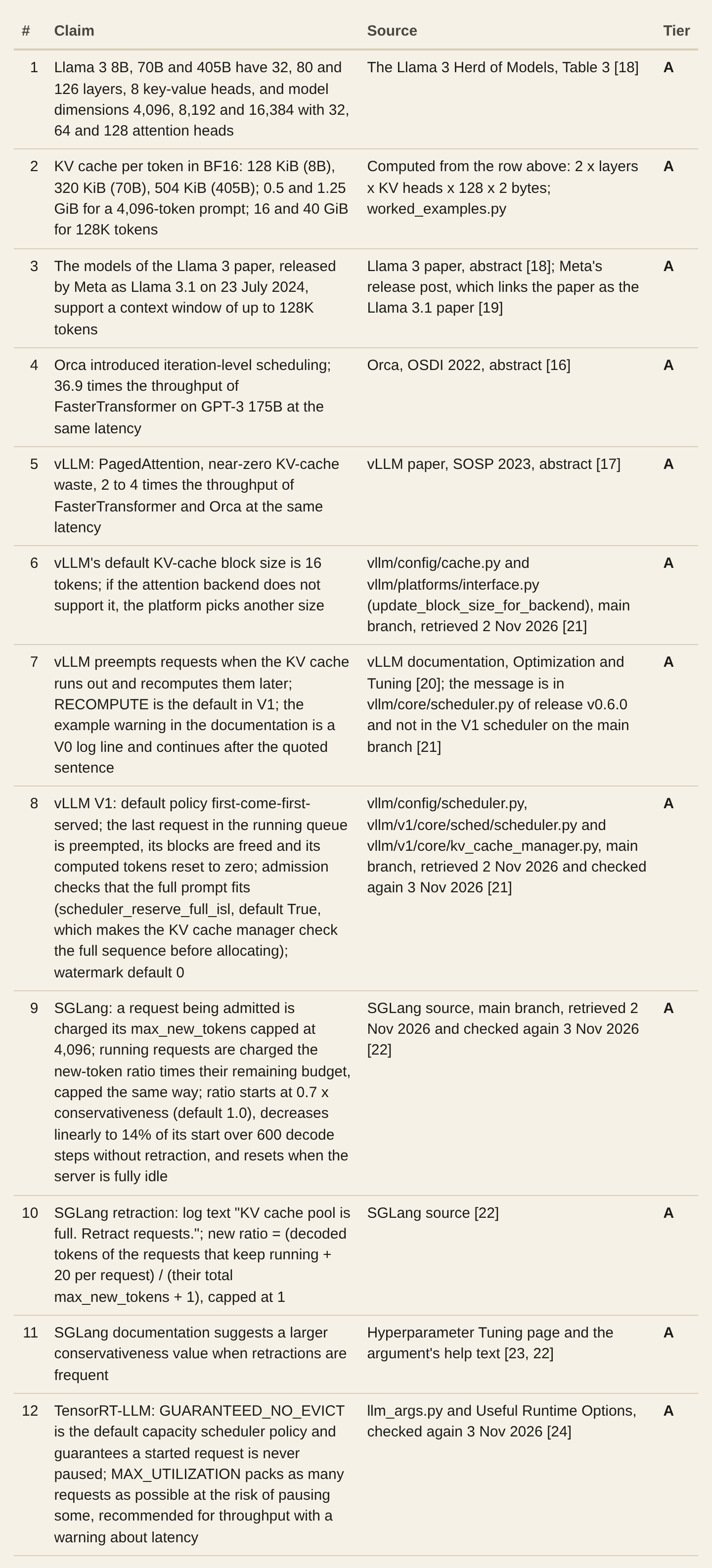
The size per token is simple arithmetic: two tensors, keys and values, per layer, each holding one vector per key-value head. For Llama 3 8B, Table 3 of the Llama 3 paper lists 32 layers, a model dimension of 4,096, 32 attention heads and 8 key-value heads, the last number being the effect of grouped query attention.
The head dimension is 4,096 / 32 = 128. In BF16, at two bytes per number, one token costs 2 × 32 × 8 × 128 × 2 = 131,072 bytes, which is 128 KiB. Llama 3 70B has 80 layers and the same 8 key-value heads of dimension 128, so it costs 320 KiB per token. The 405B model has 126 layers and costs 504 KiB per token.
Multiply by a prompt and the numbers stop being small. A 4,096-token prompt occupies 0.5 GiB of KV cache on the 8B model and 1.25 GiB on the 70B model before the first output token exists.
A full 128K-token context, the maximum the Llama 3 paper reports for its models, which Meta released as Llama 3.1, needs 16 GiB on the 8B model and 40 GiB on the 70B model.
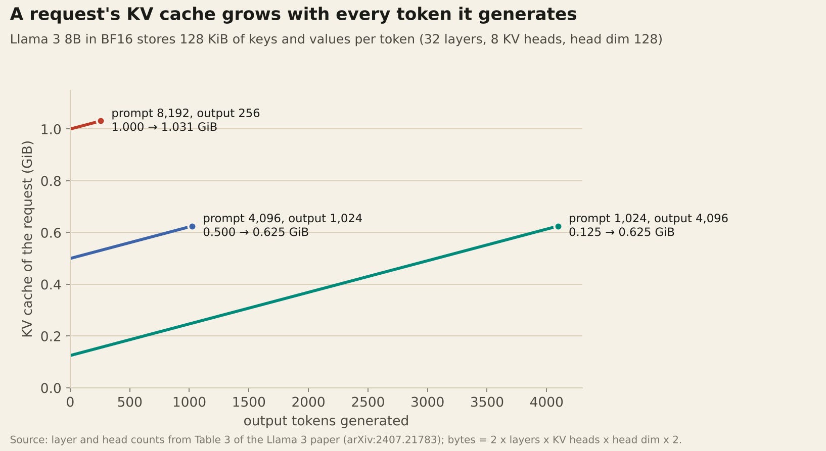
The word that matters is per token. A request is not a fixed block of memory. It starts at the size of its prompt and grows by one token’s worth of KV cache at every step until it finishes. In the chart, the request with a 1,024-token prompt and a 4,096-token answer starts at 0.125 GiB and ends at 0.625 GiB.
Orca, presented at OSDI 2022 by Gyeong-In Yu and coauthors, introduced iteration-level scheduling: the server decides at every decode step which requests are in the batch, so a finished request leaves immediately and a new one can join without waiting for the whole batch to drain. Its abstract reports a 36.9 times throughput improvement over NVIDIA FasterTransformer on GPT-3 175B at the same latency.
vLLM, presented at SOSP 2023 by Woosuk Kwon and coauthors, introduced PagedAttention, which stores the KV cache in fixed-size blocks in the way an operating system stores memory in pages, so a request no longer needs one contiguous region.
The vLLM paper reports near-zero waste in KV-cache memory and 2 to 4 times the throughput of FasterTransformer and Orca at the same latency. In vLLM’s current code the default block holds 16 tokens, unless the attention backend requires another size.
Paging nearly eliminates fragmentation, but the scheduler still has to decide which requests to admit. A scheduler that admits many requests now fills the GPU, but every one of them keeps growing, and a few hundred steps later the cache can run out.
Admit too few and the GPU idles. vLLM’s documentation describes what happens when the cache does run out: the engine preempts requests to free space, and in the V1 engine the default is to recompute them later rather than swap them to CPU memory.
The example warning on that page, a log line from the older V0 engine, begins: “Sequence group 0 is preempted by PreemptionMode.RECOMPUTE mode because there is not enough KV cache space.”
In the scheduler code on the main branch, under the default first-come-first-served policy, the request that gets preempted is the last one in the running queue, and it has to rebuild its KV cache before it can continue.
So every serving engine answers, at every step, the same question: which waiting requests should start now, given how big they will become?
The model
The model most of the recent theory uses comes from Patrick Jaillet, Jiashuo Jiang, Konstantina Mellou, Marco Molinaro, Chara Podimata and Zijie Zhou, in a paper first posted in February 2025 and now in its fifth version. It keeps the part of the problem described above and leaves out almost everything else.
Time runs in rounds, and one round is one decode step for the whole batch. Request i has a prompt of si tokens and an output of oi tokens. Once started, it is processed in oi consecutive rounds and produces one token per round; the prompt is processed in the same round as the first output token.
While it produces its j-th output token it occupies si + j units of memory, its prompt plus everything generated so far. Any number of requests can share a round as long as their memory adds up to at most M. Requests are not preempted: once started, a request runs to completion.
The objective is the total end-to-end latency, TEL, the sum over requests of the time from arrival to completion.
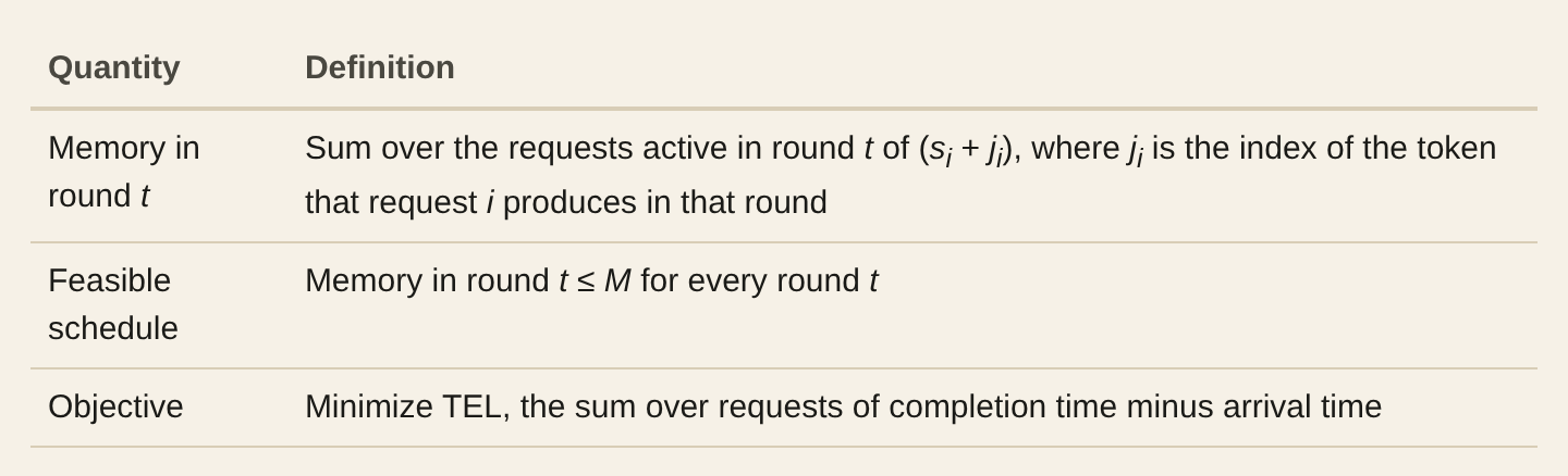
The model leaves out chunked prefill, which splits a long prompt over several rounds, the fact that a round with more tokens takes longer, prefix sharing between requests, the block granularity of the cache, multiple GPUs, and preemption with recomputation.
Each of these matters in practice. Leaving them out is what makes the model analyzable. A richer model that contains this one as a special case inherits any hardness proved here; a richer model that changes the rules has to be looked at on its own.
The version this post is about is the offline one: all requests are available at time zero and their output lengths are known in advance. Real schedulers know neither the future arrivals nor the output lengths. But if the offline version cannot be solved exactly in polynomial time, then no amount of information about the future makes exact scheduling easy.
The offline optimum is also the yardstick: Jaillet et al. measure their online algorithm against a hindsight-optimal benchmark that they write as an integer program, and they note that solving it is expensive, which is why their comparison with it uses small synthetic instances.
What vLLM, SGLang and TensorRT-LLM do
The model assumes a scheduler that knows every output length and never preempts. Real engines do not know the output lengths, and three widely used open-source engines hedge against that in different ways. The descriptions below come from their code and documentation as of 2 November 2026.
vLLM admits optimistically. Before admitting a request, its V1 scheduler checks that the whole prompt fits in the free KV-cache blocks, through an option called scheduler_reserve_full_isl that is on by default, and it reserves nothing for the output the request will generate.
A watermark that keeps a fraction of the blocks free does exist, but its default value is zero. When a running request needs a new block and none is free, the scheduler preempts: under the default first-come-first-served policy it removes the last request in the running queue, frees its blocks, and later recomputes its KV cache, prompt and generated tokens included, once space is available again. vLLM thus accepts the risk of running out of memory and pays for it with recomputation.
SGLang estimates. When it decides whether a new request fits, it charges that request its prompt plus its max_new_tokens budget, capped at 4,096 tokens, but it charges each request that is already running only a fraction of its remaining budget, capped the same way.
The fraction is a new-token ratio that starts at 0.7 times a conservativeness parameter, which defaults to 1.0. It decreases by a fixed step at every decode step in which no request is retracted, reaches a floor of 14% of its starting value after 600 such steps, and returns to the starting value whenever the server is fully idle.
When the cache fills up anyway, SGLang retracts running requests, logs “KV cache pool is full. Retract requests.”, and resets the ratio to an estimate computed from the requests that keep running: the tokens they have decoded so far, plus 20 per request, divided by one more than their combined max_new_tokens, and capped at 1.
Its documentation suggests raising the conservativeness parameter if requests are retracted often. SGLang therefore predicts how much the running requests will still grow and corrects the prediction when it turns out wrong.
TensorRT-LLM reserves. Its default capacity scheduler policy, GUARANTEED_NO_EVICT, is designed to guarantee that a started request is never paused, so it has to be conservative about the memory each request will need later.
The alternative, MAX_UTILIZATION, packs as many requests as possible at each iteration, at the risk of pausing requests when the KV-cache limit is reached; NVIDIA’s tuning guide recommends it for throughput and warns that pauses can hurt latency.
These are three answers to the question the model formalizes: how much future growth to plan for when admitting a request. The offline model studied here sits at the reserving end, with perfect knowledge of the output lengths.
MC-SF, the memory-constrained shortest-first algorithm of Jaillet et al., admits a request only if the projected memory of everything running, computed from the predicted output lengths, stays within the budget in every future round. The result in this post says that even at that end, with exact lengths and no arrivals, finding the best admission schedule is NP-hard.
Two years of results
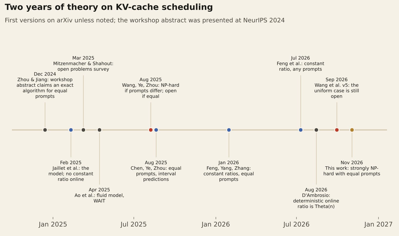
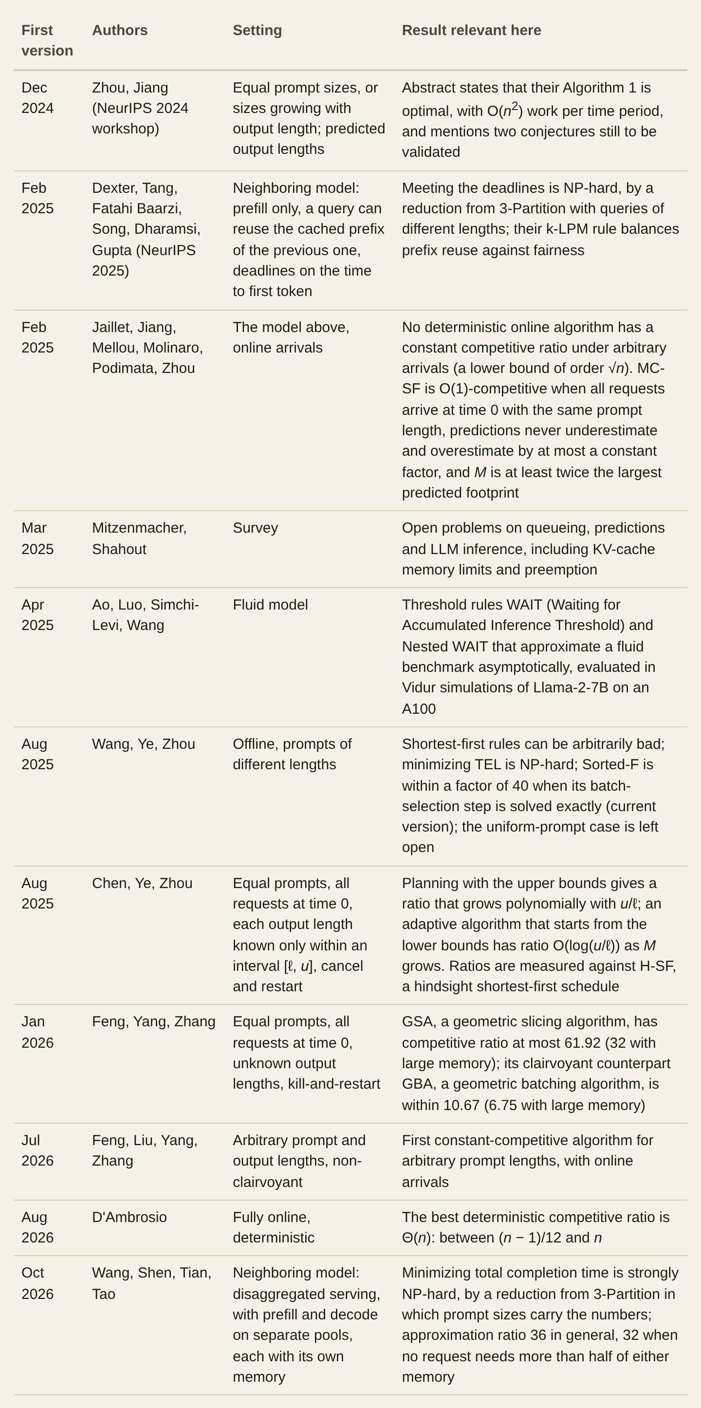
The theory on this model is young: almost all of it appeared on arXiv in the last two years. The timeline shows the papers on this model, with the date of their first public version. The table gives their results as they stand in the current versions and adds two hardness results for neighboring models.
A few terms recur in these papers. An algorithm that has to decide without some of the information, future arrivals or output lengths, is judged by its competitive ratio: the worst case, over all inputs, of its cost divided by the cost of an optimal schedule computed with full knowledge.
For an algorithm that knows everything in advance and whose only limit is a polynomial running time, the same ratio is called its approximation ratio. A clairvoyant scheduler knows each output length when the request arrives; a non-clairvoyant one finds it out only when the request finishes.
In the kill-and-restart model a scheduler may abort a running request, throw away its KV cache and the tokens it has generated, and start it again from scratch later.
A fluid benchmark replaces individual requests with a continuous flow of work and gives a target that good policies approach as the system grows. Vidur is a simulator of LLM inference that predicts the running time of each model operation from profiling data.
A separate line of work uses queueing models and asks how much traffic a server can sustain, rather than how to schedule a given batch.
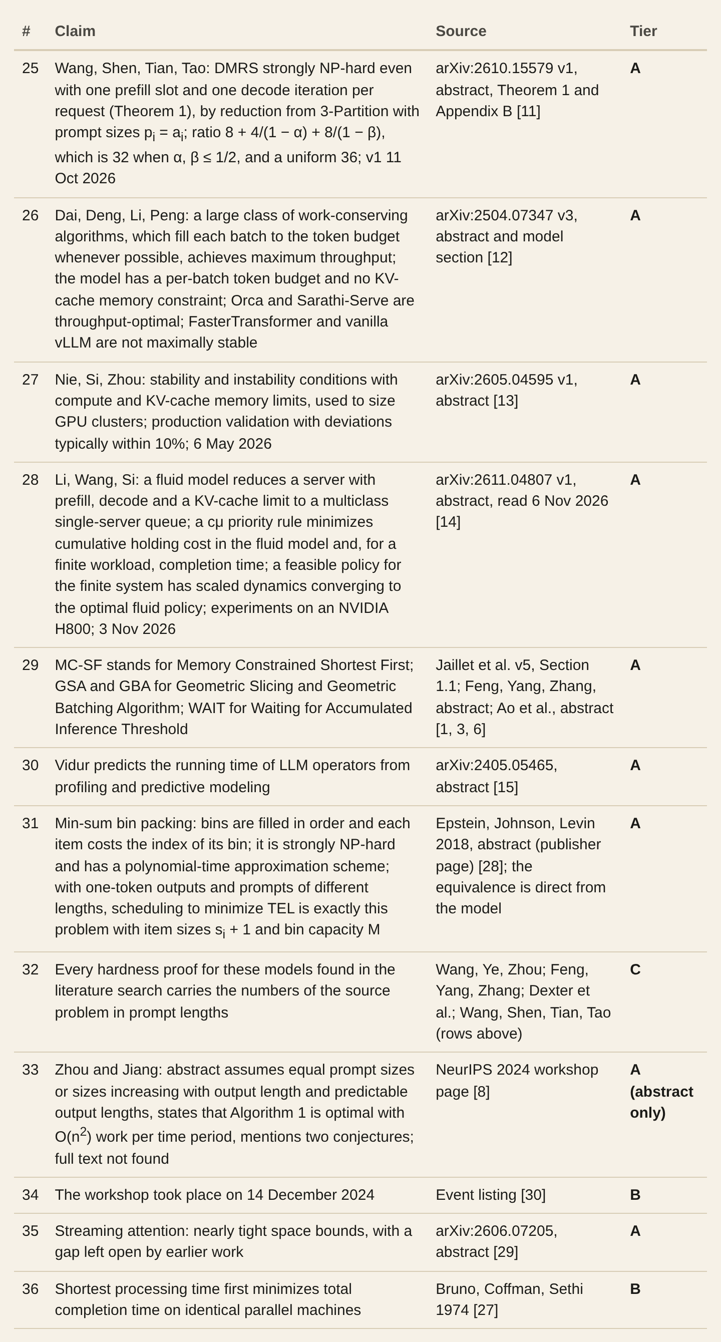
In a model with a token budget per batch and no memory constraint, Dai, Deng, Li and Peng show that a broad class of work-conserving schedulers, which fill every batch to the budget whenever enough work is waiting, reaches maximum throughput; in their analysis Orca and Sarathi-Serve, a scheduler built around chunked prefill, are throughput-optimal, while FasterTransformer and vanilla vLLM are not maximally stable.
Nie, Si and Zhou add the KV-cache memory limit, derive conditions under which a server stays stable, and propose using them to size GPU clusters; in tests on production GPUs their predictions deviated from measurements typically by less than 10%.
Most recently, on 3 November 2026, Li, Wang and Si modeled a server with a KV-cache limit as a multiclass fluid queue, proved that a cμ priority rule, which favors the class with the largest product of holding cost and service rate, is optimal for the fluid model, and built policies for the finite system that converge to it; on an NVIDIA H800 their rule substantially reduced average latency.
Results of this kind describe behavior at scale, not the exact optimum of a given batch, so they do not conflict with the hardness result below.
MC-SF and Sorted-F show what a good heuristic looks like here. MC-SF scans the waiting requests in order of predicted output length and admits them one by one as long as the projected memory of everything running, computed from the predictions, stays within the budget in every future round; it stops at the first request that does not fit.
Sorted-F, the algorithm of Wang, Ye and Zhou, first builds an ordered list by repeatedly picking the feasible batch that minimizes the sum of its output lengths divided by the square of its size, which favors large batches of short requests, and then admits the longest prefix of that list that fits, at every round.
Both are admission rules with a look-ahead on memory, and both are provably within a constant factor of the optimum in their settings. For Sorted-F, the factor 40 assumes that each batch of the first phase is chosen exactly.
The paper does this with a dynamic program whose running time grows with the memory size, for batches whose peak footprints, added up, fit in memory; the factor 40 also holds under that stricter rule.
The constant-factor guarantees for MC-SF and for the geometric algorithms of Feng, Yang and Zhang are proved for identical prompts. Feng, Yang and Zhang make that assumption to isolate the algorithmic difficulty, and they point out that with prompts of different lengths the one-token case is already strongly NP-hard, through min-sum bin packing, a version of bin packing in which the bins are filled in order and each item costs the position of its bin.
Both hardness results for this model, the NP-hardness proof of Wang, Ye and Zhou and the min-sum bin packing observation of Feng, Yang and Zhang, need prompts of different lengths.
So do the two hardness results for neighboring models in the table: Dexter and coauthors encode 3-Partition in the lengths of queries, and Wang, Shen, Tian and Tao in the sizes of prompts.
In every hardness proof for these models that we could find, the numbers of the source problem are carried by prompt lengths. Sorted-F and the 2026 scheduler of Feng, Liu, Yang and Zhang handle arbitrary prompts, so they cover identical ones too. What remained open was whether identical prompts make exact optimization tractable.
Hardness, in one page
A short reminder of the vocabulary. A problem is in P if some algorithm solves every instance in time polynomial in the size of the input. A problem is NP-hard if a polynomial-time algorithm for it would give polynomial-time algorithms for every problem in NP, which almost everyone believes is impossible.
The standard way to prove NP-hardness is a reduction: take a problem already known to be hard and show how to translate any of its instances, in polynomial time, into an instance of your problem with the same answer.
Numbers create a subtlety. Some problems with numbers are hard only because the numbers can be huge. The textbook example is knapsack, which is NP-hard but can be solved by a dynamic program in time proportional to the number of items times the capacity, which is fast when the capacity is small.
Such an algorithm is called pseudo-polynomial: polynomial in the magnitude of the numbers, not in the number of digits needed to write them down. A problem is strongly NP-hard if it stays NP-hard even when all its numbers are bounded by a polynomial in the size of the input. Unless P = NP, a strongly NP-hard problem has no pseudo-polynomial algorithm.
For KV-cache scheduling the distinction is practical. The numbers in an instance are token counts, and the memory budget is measured in tokens: hundreds of thousands to millions, depending on the model and the hardware.
A dynamic program with one table entry per possible amount of used memory would be pseudo-polynomial and might well be fast enough in practice. Strong NP-hardness says that no such exact algorithm exists unless P = NP.
Under the same assumption it also rules out a fully polynomial-time approximation scheme, an algorithm that gets within any chosen factor 1 + ε of the optimum in time polynomial in the input and in 1/ε, because running it with ε small enough would return the exact optimum in pseudo-polynomial time. Garey and Johnson spelled out these consequences in 1978.
The starting point of the reduction is 3-Partition: given 3m positive integers, each larger than a quarter and smaller than half of a target B, with total mB, can they be split into m triples that each sum to exactly B? Garey and Johnson proved it strongly NP-complete in 1975, in a paper about multiprocessor scheduling under resource constraints, and it remains a standard tool for showing that scheduling problems with resources are strongly NP-hard.
Its relative, bin packing, asks whether items fit into m bins of capacity B; it contains 3-Partition as a special case and is strongly NP-complete too.
The footnote
The question sits in footnote 1 of the paper by Wang, Ye and Zhou, attached to the sentence where they say the problem becomes computationally hard without uniform inputs:
Whether minimizing TEL is NP-hard under uniform si remains open.
The first version, posted in August 2025, already raised the question in a footnote worded differently, and it is still open in the fifth version, posted on 29 September 2026.
To see why the question is not trivial, look at how their hardness proof works. They take an instance of 3-Partition, a classic strongly NP-complete problem that asks whether 3m numbers can be split into m triples with the same sum T.
Each number xi becomes a request with prompt length xi and a single output token, and the memory is set to M = T + 3. A one-token request occupies xi + 1 units for exactly one round, so filling each round to capacity means packing numbers into bins. Scheduling becomes bin packing, and the prompt lengths carry all the information.
With a common prompt length, that proof has nothing to hold on to. Every one-token request is now identical, and the best schedule for identical one-token requests is obvious: put as many as fit in every round. All the combinatorial information has to live in the output lengths.
An output length controls how long a request stays and how far its memory ramps up, but every request ramps up at the same rate, which leaves far less room to encode numbers than a prompt length does.
There were other reasons to expect the uniform case to be easier. The closest classical problem, minimizing total completion time on identical parallel machines, is solved exactly by the shortest-processing-time rule (Bruno, Coffman and Sethi, 1974).
MC-SF is a shortest-first rule and it has a constant-factor guarantee for identical prompts. And a workshop abstract from December 2024 claims an exact algorithm for the equal-size case.
Lanes
The proof starts from a change of viewpoint. With a common prompt length s, the memory in any round splits into two parts:

Now suppose the prompt is long compared with the outputs, and write the budget as M = k·s + R with a remainder R smaller than s. Three things happen at once.
No set of k + 1 requests ever fits, because their prompts alone take (k + 1)s, which is more than M. Any k − 1 requests always fit, provided outputs are short enough that k − 1 of them can never accumulate more than s tokens of decode load. And exactly k requests fit precisely when their token indices add up to at most R.
The paper calls this the lane lemma. The GPU behaves like k parallel lanes, and the last lane is open only while the active requests are young, that is, while they have produced few tokens.
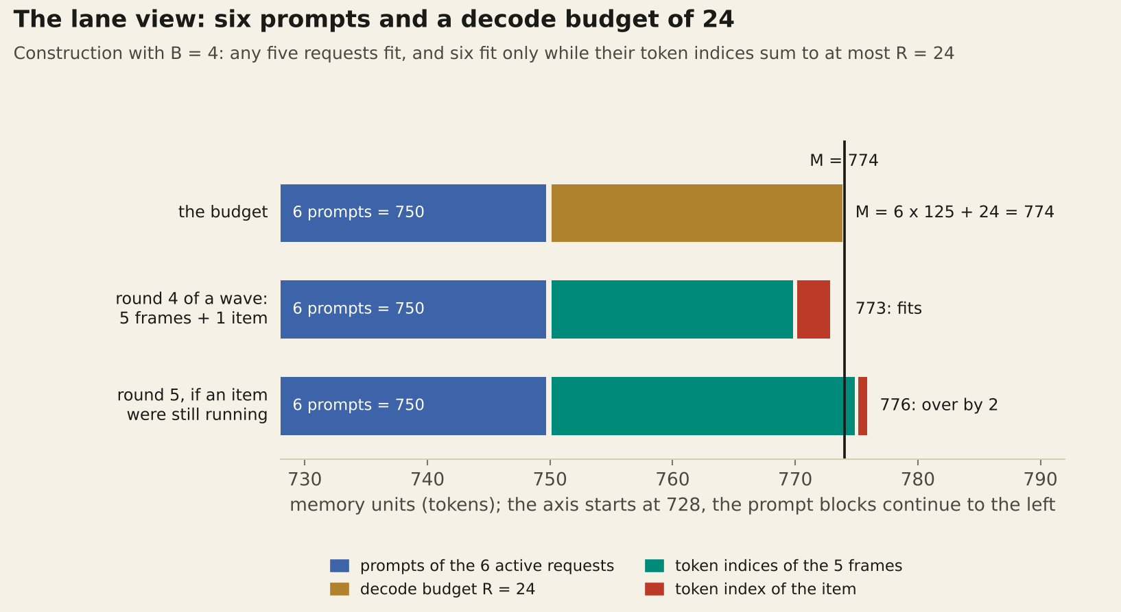
The two extreme budgets show where the difficulty lives. If R is smaller than k, then k requests can never be active together, because each token index is at least 1. The problem becomes scheduling on k − 1 identical machines, and shortest-first is optimal.
If R is at least k times the longest output, the budget never binds. The problem becomes scheduling on k identical machines, and shortest-first is optimal again. Everything interesting happens in between, when the last lane opens and closes depending on how old the requests on the other lanes are.
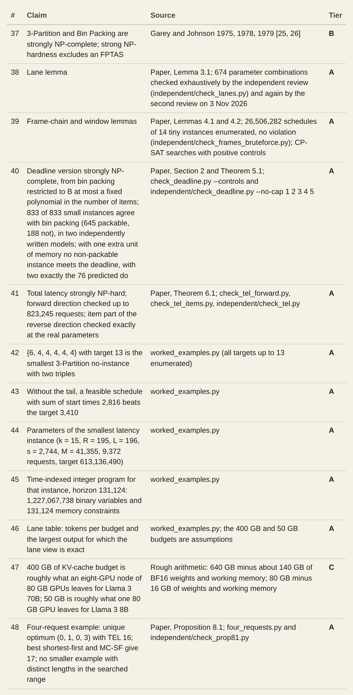
The regime requires prompts at least k − 1 times longer than the longest output, where k is the largest number of requests that can be active at once. For a sense of scale, take Llama 3 70B in BF16, 320 KiB per token, and suppose that 400 GB of GPU memory, 4 × 1011 bytes, are left for the KV cache, roughly what a node of eight 80 GB GPUs leaves after the 140 GB of weights and some working memory.
That budget holds 1,220,703 tokens. For the 8B model the table assumes 50 GB, roughly what a single 80 GB GPU leaves after 16 GB of weights. If every prompt has the same length, the lane view is exact for outputs up to the length in the last column:
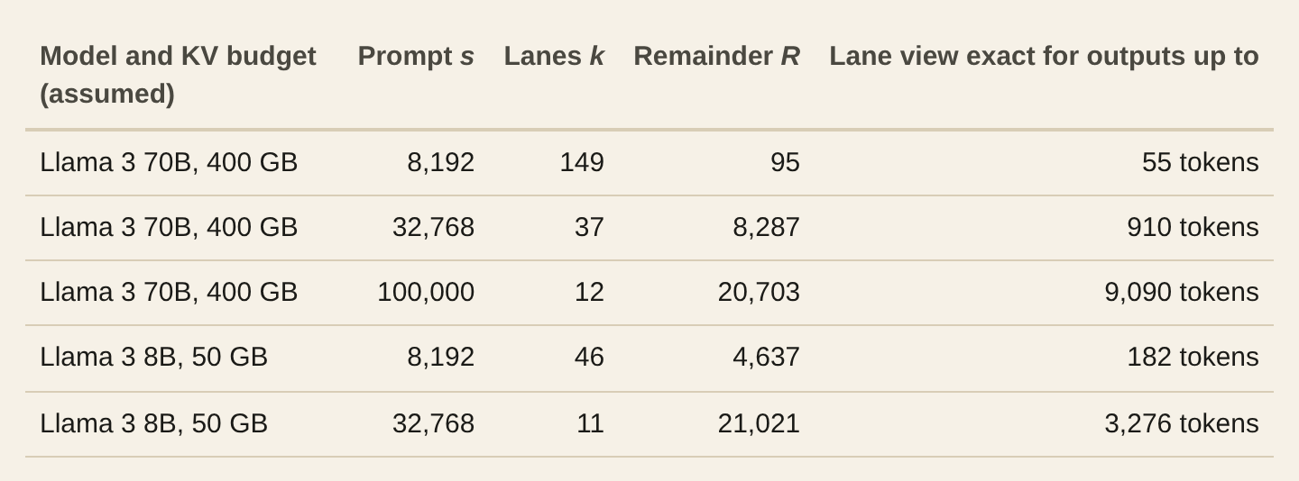
Chat traffic, with short prompts and answers of hundreds of tokens, does not look like the first row. Long-context work does look like the later rows: with 100,000-token documents only twelve requests fit on that node, and any answer up to 9,090 tokens keeps the lane view exact, well within the 128K-token context of the 70B model in its Llama 3.1 release.
By this measure, summarizing long documents and answering questions over a large retrieved context are the workloads closest to the hard regime. The regime is realistic; the hard instances themselves, with their synchronized waves of identical requests, are artificial, as the instances built in reductions usually are.
Waves and windows
The reduction uses two kinds of requests. Frames are long requests, all with the same output length L. Items are short requests whose output lengths are the numbers of the problem we want to encode. The parameters are chosen as functions of the bin capacity B of that problem:
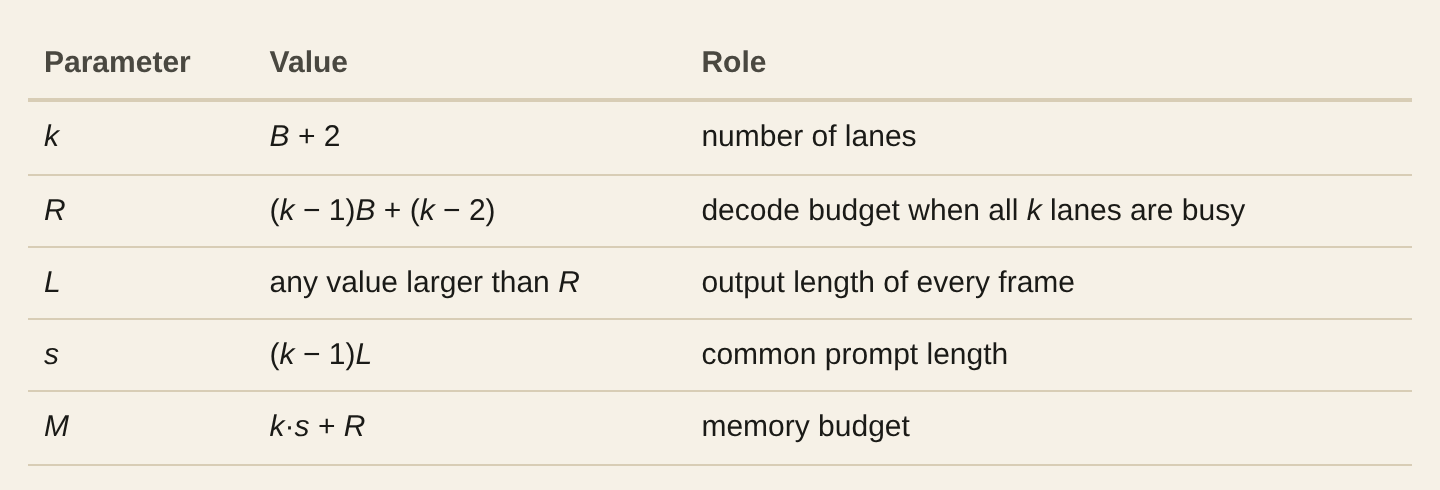
The first fact is that k frames can never run at the same time. If they did, look at the first round in which one of them is about to finish. In that round it has token index L, the others have index at least 1, and their sum is more than R. So frames effectively use at most k − 1 lanes.
A consequence is that frames form chains: if the frames are sorted by start time, frame number r + k − 1 cannot start before frame r ends. The cheapest way to run the frames is in synchronized waves of k − 1, starting at times 0, L, 2L, and so on, and any frame that starts late drags every later frame in its chain with it.
The second fact is the window. In round j of a wave the k − 1 frames all have token index j, so a k-th request can run only if its own token index α satisfies (k − 1)j + α ≤ R.
Since every item has length at most B = k − 2, its index is between 1 and k − 2, and with the value of R above the inequality holds exactly when j ≤ B. In round B + 1 even an item with index 1 needs (k − 1)(B + 1) + 1 = (k − 1)B + k, which is two more than R.
Every wave therefore opens a window of exactly B rounds at its start, and inside a window items run one at a time. The items placed in a window can have total length at most B, and any set of items with total length at most B can be placed there back to back.
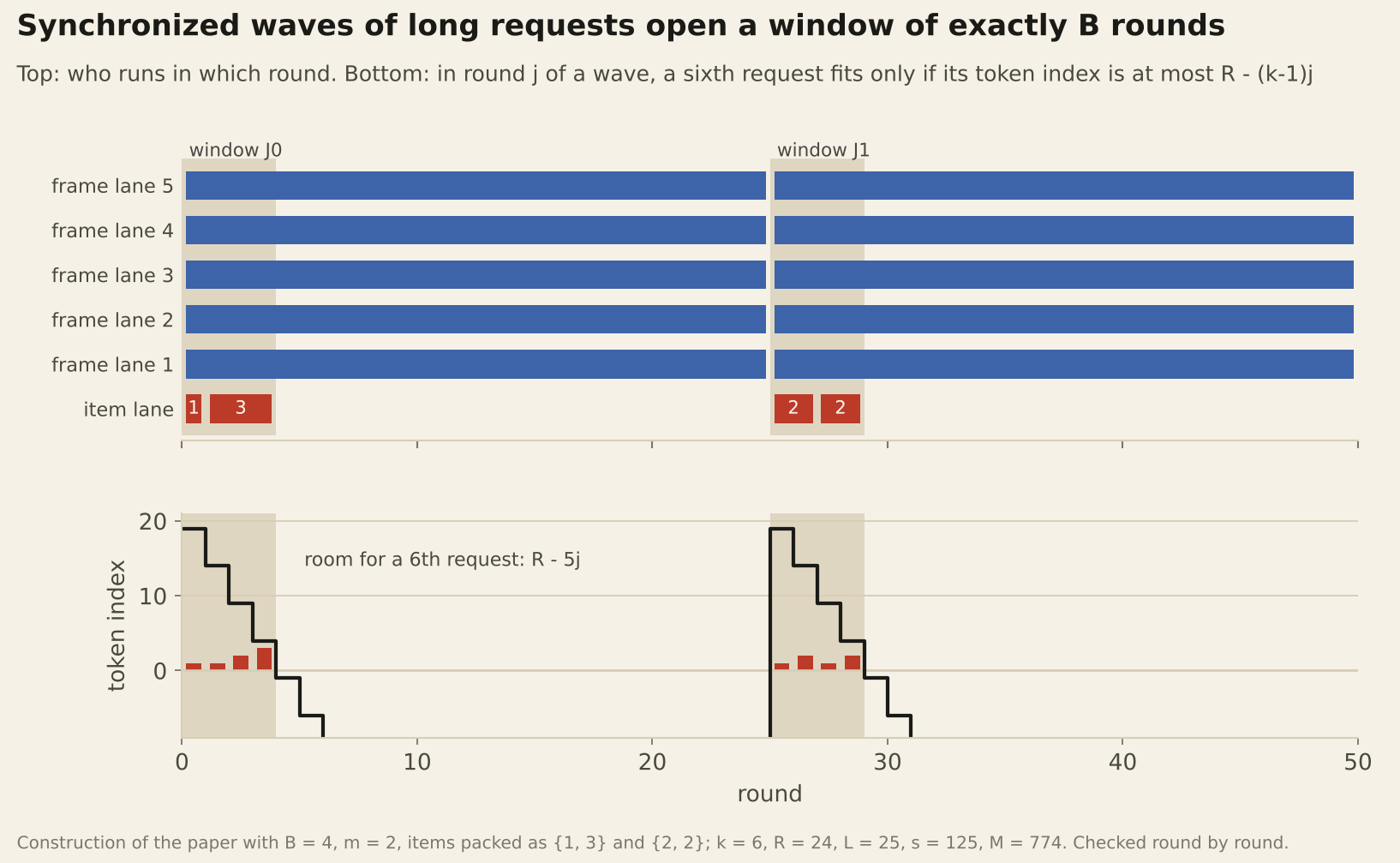
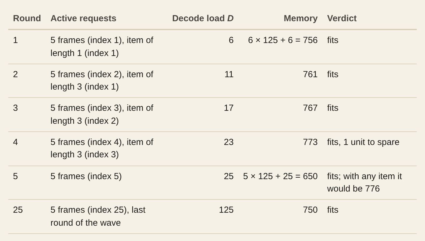
In the small instance of the figure, s = 125 and M = 774. The first wave starts at time 0, and its window holds an item of length 1 followed by an item of length 3:
From windows to bin packing
For the deadline version, take a bin packing instance: item sizes, a capacity B, and m bins. Build the instance above with L = R + 1, m waves of frames, and one item request per item, and ask whether every request can finish by time mL.
If the items fit into m bins, put the content of bin w into the window of wave w, and every request finishes by mL. Conversely, if every request finishes by mL, the chain property forces every frame to start exactly at the beginning of its wave, because the last frame of each chain must start by (m − 1)L and each step of the chain costs L rounds.
With the frames pinned, every item must sit inside some window, and the windows are bins of capacity B. So deciding whether a batch of LLM requests with identical prompts can finish by a deadline is at least as hard as bin packing, which is strongly NP-complete. All numbers in the construction are polynomial in the input (L = B2 + 2B + 1, s = (B + 1)L), which is what makes the hardness strong.
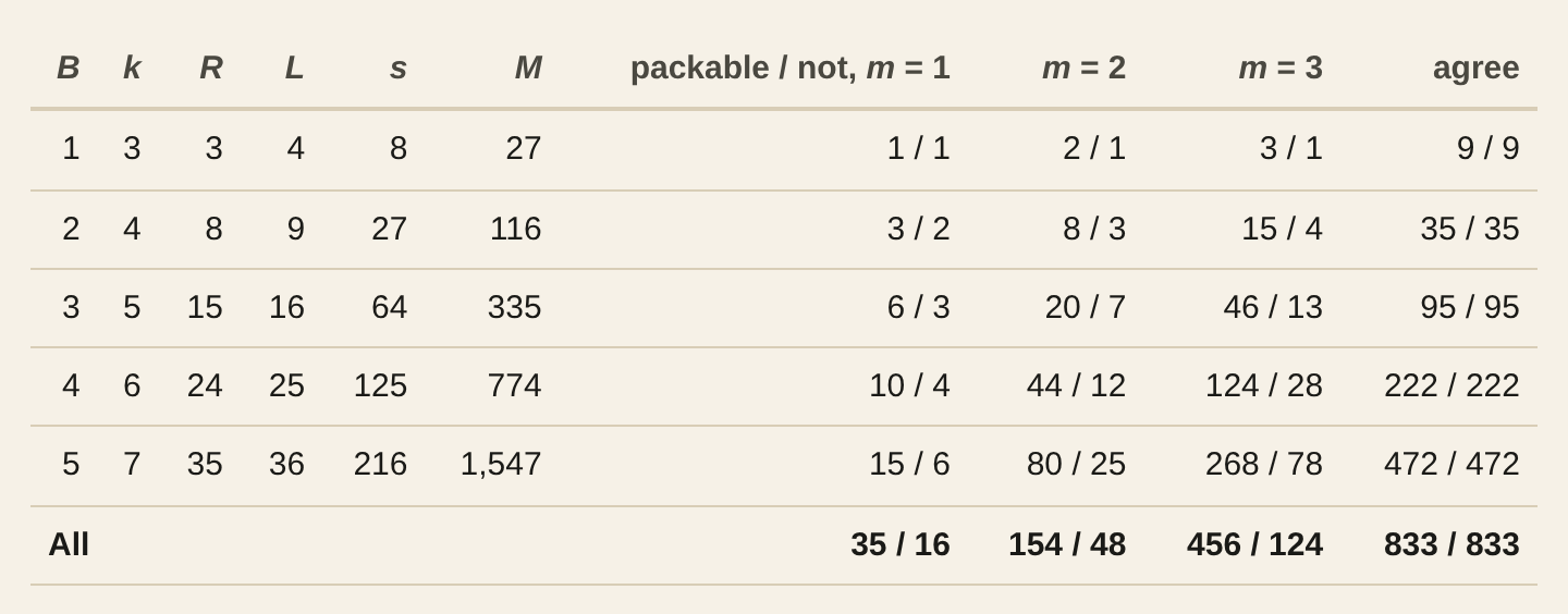
This part of the argument can be tested end to end. For every bin capacity B from 1 to 5 and every number of bins m from 1 to 3, every multiset of at most 2m + 1 item sizes between 1 and B with total at most mB + 1 was enumerated, 833 instances in total, 645 packable and 188 not.
For each one, the constructed scheduling instance was solved exactly with Google’s CP-SAT solver, asking whether any schedule at all satisfies the memory constraint in every round and finishes by mL. The answer matched exhaustive bin packing on all 833, and a second model, written independently, gave the same 833 answers.
A check like this is worth something only if it could have failed, so the 188 non-packable instances were solved again with slightly more memory. The arithmetic of the windows predicts what should happen.
One extra unit of memory changes nothing, because a window still closes after B rounds. Two extra units add one round to every window, and in that round an item can run only if it has length 1 and starts there.
With two extra units, then, an instance should meet the deadline exactly when its items split into m groups of total at most B, or B + 1 for a group that contains an item of length 1. The solver found no schedule with one extra unit, and with two it found schedules for exactly the 76 instances that this rule predicts.
It finds schedules beyond bin packing as soon as the construction allows them, and the construction turns out to have exactly one unit of memory to spare.
Total latency and the tail
The open question was about total latency, not deadlines, and total latency is slipperier. A schedule is no longer judged on whether it meets a date but on the sum of all completion times, and a clever schedule might give up a little on some requests to gain a lot on others.
The obvious temptation in this construction is to run the items first. Items are short and can run many at a time when the frames are not there, so starting all of them at time 0 and delaying the frames slightly can be much cheaper than making each item wait for its window.
Take the smallest no-instance of 3-Partition, the six numbers 6, 4, 4, 4, 4, 4 with target 13: a triple that contains the 6 sums to 14 and a triple without it sums to 12, and no instance with two triples and a smaller target is a no-instance.
Build the construction with only the two waves the items need. The target on the sum of start times is then 3,410. But the schedule that starts all six items at time 0 together with eight frames, starts the other six frames of the first wave at time 6, and repeats the same pattern for the second wave at times 196 and 202 is feasible, because never more than 14 = k − 1 requests are active at once, and its sum of start times is 2,816.
It beats the target although no 3-partition exists. Without something more, the reduction would be wrong.
The fix is a long tail of extra frame waves after the m that the items use. Because frames form chains, delaying one frame of an early wave by one round delays every later frame in its chain by at least one round, so with T extra waves the penalty is at least T. The paper sets the parameters as follows.
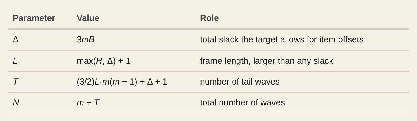
These values make the tail penalty larger than anything the items could possibly gain. Any schedule that meets the target must keep the first m + 1 waves exactly aligned, and then every item sits in a window, starting no earlier than L times the index of its window.
A window holds at most three items, because in 3-Partition every number is larger than a quarter of the target. If the 3-partition exists, the items fill the first m windows three at a time and the cost stays under the target.
If it does not, some window among the first m has fewer than three items, at least one item is pushed into a later window, and the sum of window indices goes up by at least 1, which costs at least L. Since L is larger than Δ, the total slack the target allows for item offsets, the cost goes over.
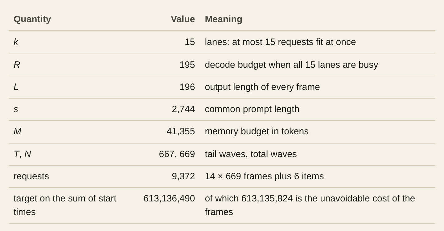
The instances are large but polynomial. For the smallest no-instance above, the construction has these parameters:
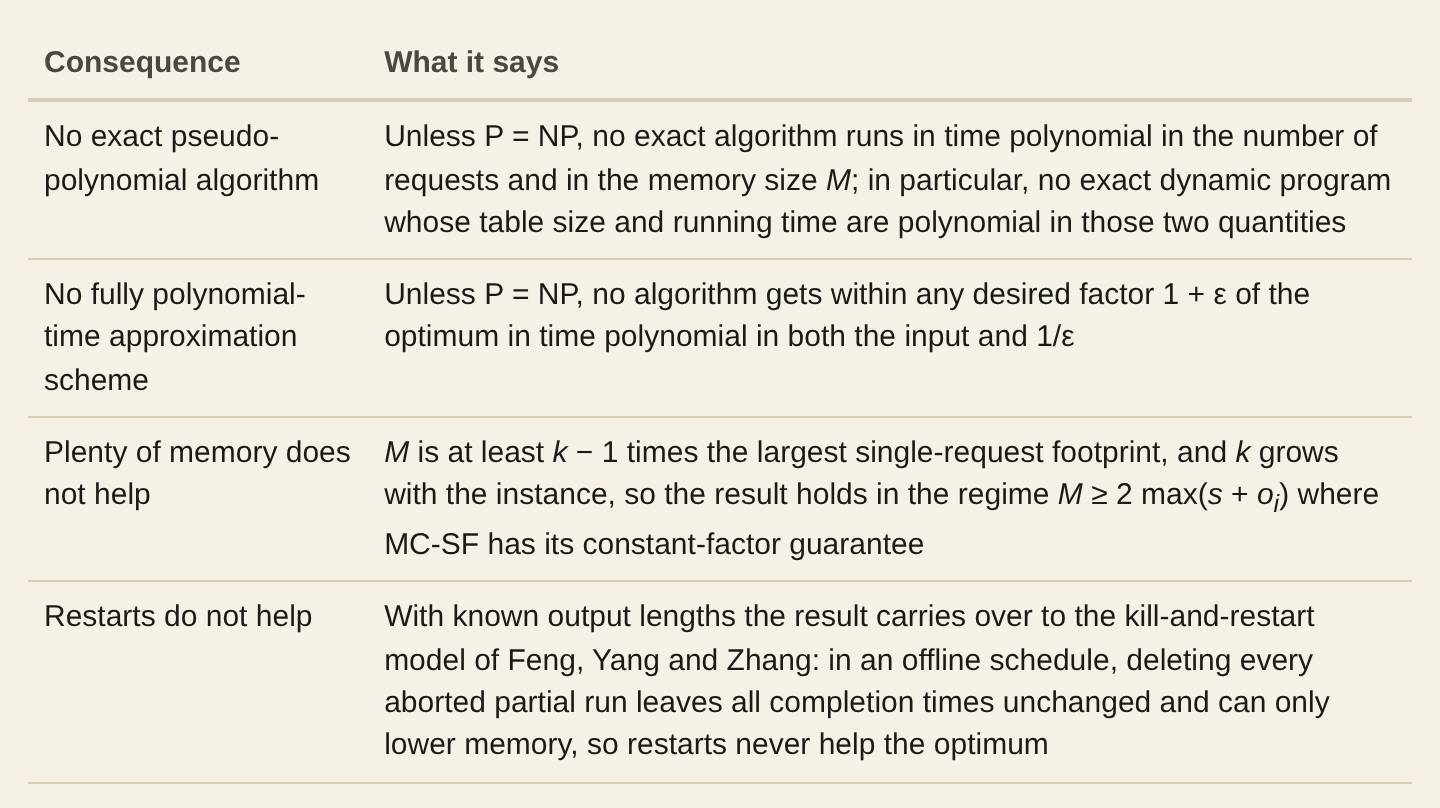
Strong NP-hardness and the shape of these instances have four consequences.
Four requests
The reduction needs thousands of requests, but the failure of the simplest rule shows up much earlier. Take a common prompt of 3 tokens, a budget of 11 units, and four requests with output lengths 1, 2, 4 and 5.
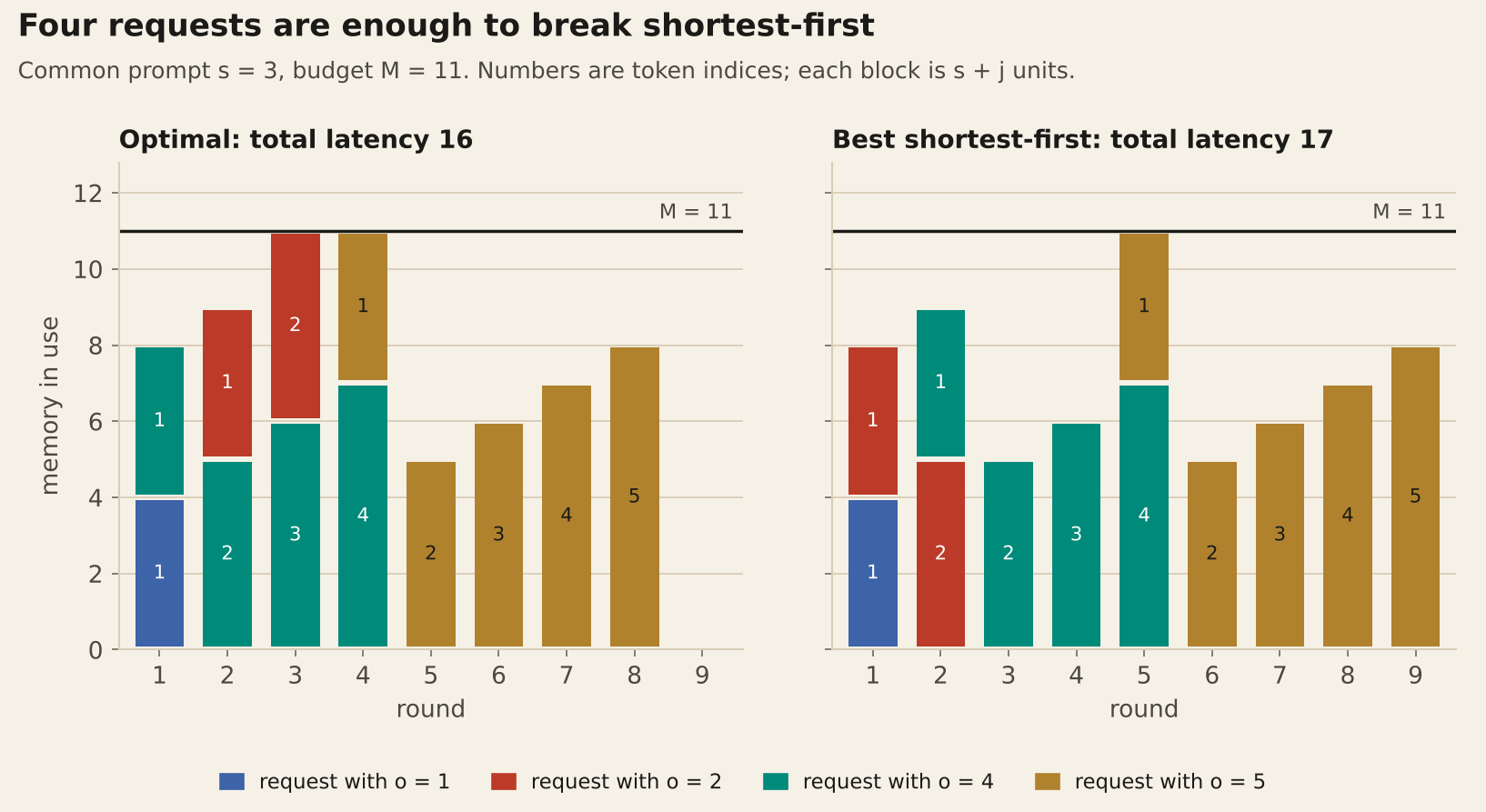
Three requests never fit together here, since three prompts and three first tokens already need 12 units, and two requests fit together only while their token indices sum to at most 5.
The two long requests, of lengths 4 and 5, cannot overlap much: one can start at most one round before the other ends. The optimal schedule starts the length-4 request at time 0, next to the length-1 request, slips the length-2 request in at time 1, and starts the length-5 request at time 3, so that it overlaps only the last round of the length-4 request.
Total latency 16. A schedule that starts requests in order of output length cannot start the length-4 request at time 0, because the two shorter requests would also have to start at time 0 and three requests never fit; that pushes the length-5 request to time 4. Total latency 17.
Exhaustive search confirms that (0, 1, 0, 3) is the only optimal vector of start times, and that MC-SF, as described in Algorithm 1 of Jaillet et al., outputs (0, 0, 1, 4). H-SF, the hindsight schedule against which Chen, Ye and Zhou measure their ratios, starts at every step as many waiting requests as fit.
When it breaks ties toward shorter requests, as its name says, it makes the same choices as MC-SF and also costs 17; it reaches 16 only with a tie-break that starts the length-4 request ahead of the length-2 one. These runs use the accounting of this post.
Chen, Ye and Zhou charge one token less while a token is produced, and in their accounting the same instance has a prompt of 4 tokens, with the same schedules and the same costs. A ratio measured against H-SF can therefore differ from a ratio against the optimum, and the optimum is the quantity this result shows to be NP-hard to compute.
Among all instances with three or four requests, distinct output lengths up to 7, prompt lengths from 1 to 6 and budgets up to three times the largest footprint, an exhaustive search found no example with three requests or with a smaller total output length.
With ties allowed the effect even appears with a one-token prompt: for s = 1, M = 5 and output lengths 1, 1, 3, 3, the optimum is 12 and every shortest-first schedule costs at least 13.
The proof, statement by statement
The statements and their numbers are those of the paper. A request started at time p is active in rounds p + 1 through p + o, and in round t its token index is t − p. At is the set of requests active in round t and D(t) the sum of their token indices, so memory in round t equals |At|·s + D(t).
Lemma 3.1 (lanes). Let k ≥ 2 and 0 ≤ R < s, let M = ks + R, and suppose that k − 1 times any output length is at most s. Then the memory constraint holds in round t if and only if |At| ≤ k − 1, or |At| = k and D(t) ≤ R.
Proof. With at most k − 1 active requests, D(t) is at most k − 1 times the longest output, hence at most s, and memory is at most (k − 1)s + s = ks ≤ M. With exactly k, memory is ks + D(t), which is at most M exactly when D(t) ≤ R. With k + 1 or more, every token index is at least 1, so memory is at least (k + 1)s + k + 1, which is larger than ks + R because s > R.
The construction. Given a capacity B and item lengths between 1 and B, set k = B + 2 and R = (k − 1)B + k − 2, choose L > R and a number of waves N, and set s = (k − 1)L and M = ks + R. The instance has (k − 1)N frames of output length L and one item request per item. Lemma 3.1 applies because no output is longer than L.
Lemma 4.1 (frame chains). In every feasible schedule at most k − 1 frames are active in any round. If f1 ≤ f2 ≤ … are the frame start times in sorted order, then fr+k−1 ≥ fr + L, so frame r starts no earlier than wrL, where wr = ⌊(r − 1)/(k − 1)⌋ is its wave. If some frame starts later than that, the total delay of all frames is at least N − wr.
Proof. If k frames were active together, take the first round in which one of them is active for the last time. All k are active in that round, that frame has token index L, and the sum of indices is at least L + k − 1 > R, which Lemma 3.1 forbids. If fr+k−1 were smaller than fr + L, the k frames r, …, r + k − 1 would all be active in round fr+k−1 + 1. The bound wrL follows by induction. A late frame delays every later frame of its chain r, r + (k − 1), r + 2(k − 1), and so on, and the chain has N − wr members from frame r onward.
Lemma 4.2 (windows). Suppose the frames of waves 0 to W start exactly at their wave times. Then every item active in some round up to (W + 1)L runs entirely inside one window, the first B rounds of a wave; items never overlap there; and the items in a window have total length at most B.
Proof. In round wL + j the k − 1 frames of wave w are active with token index j, and no other frame is: an aligned frame of another wave is active only during its own wave, and by Lemma 4.1 a frame of a wave after W starts no earlier than (W + 1)L. An item active in that round makes k active requests, so (k − 1)j + α ≤ R with α ≥ 1, and since (k − 1)(B + 1) + 1 > R this forces j ≤ B. Rounds wL + B + 1 to (w + 1)L are therefore free of items and separate the windows, and two items can never be active in the same round.
Lemma 4.3 (filling windows). Any assignment of the items to windows with total length at most B per window can be scheduled, with the items of each window back to back and the frames in synchronized waves.
Proof. In round wL + j there are k − 1 frames of index j and at most one item, of index at most B = k − 2, and only while j ≤ B. So D ≤ (k − 1)B + k − 2 = R.
Theorem 5.1 (deadline). Deciding whether every request can finish by a given deadline is strongly NP-complete.
Proof. Reduce from bin packing with m bins of capacity B, using L = R + 1, N = m and deadline mL. A packing gives a schedule by Lemma 4.3. Conversely, meeting the deadline forces every frame to start exactly at its wave time, by following each chain backward from the last wave, and Lemma 4.2 turns the windows into bins.
Theorem 6.1 (total latency). Minimizing total end-to-end latency is strongly NP-hard.
Proof. Reduce from 3-Partition, using Δ = 3mB, L = max(R, Δ) + 1, T = (3/2)L·m(m − 1) + Δ + 1, N = m + T, and the target Kp = F* + (3/2)L·m(m − 1) + Δ on the sum of start times, where F* = (k − 1)L·N(N − 1)/2 is the cost the frames cannot avoid. A 3-partition gives a schedule below the target by Lemma 4.3, because every item starts less than B rounds after its window opens. Conversely, a schedule that meets the target has total frame delay at most T − 1, so by Lemma 4.1 the first m + 1 waves are exactly aligned. By Lemma 4.2 the items sit in windows, at most three per window, each starting no earlier than L times the index of its window, and items outside the first m + 1 windows start even later. If no 3-partition exists, the sum of the window indices exceeds its minimum value (3/2)m(m − 1) by at least one, which adds at least L > Δ to the cost and breaks the target.
Both results are strong because the reductions start from 3-Partition and bin packing instances in which B is at most a fixed polynomial in the number of items.
The two problems stay NP-complete under that restriction, which is what being strongly NP-complete amounts to for them, and every number the constructions produce, deadline and target included, is then polynomial in the number of items.
The restriction is not a formality: the constructions produce more than B requests, so without it they would not even run in polynomial time. Membership in NP is easy even with numbers written in binary: memory only needs to be checked in the rounds where some request finishes, because between two such rounds it can only grow.
How it was checked
The proofs in the paper are self-contained and use nothing beyond the definitions. Arithmetic in reductions like this one is easy to get wrong, though, so the paper and its constructions were checked in several independent ways.

The referee session’s list included one step where a definition was looser than the argument needed, a citation that was missing, and an earlier claim in the literature that conflicts with the result. The table shows each finding and what changed.
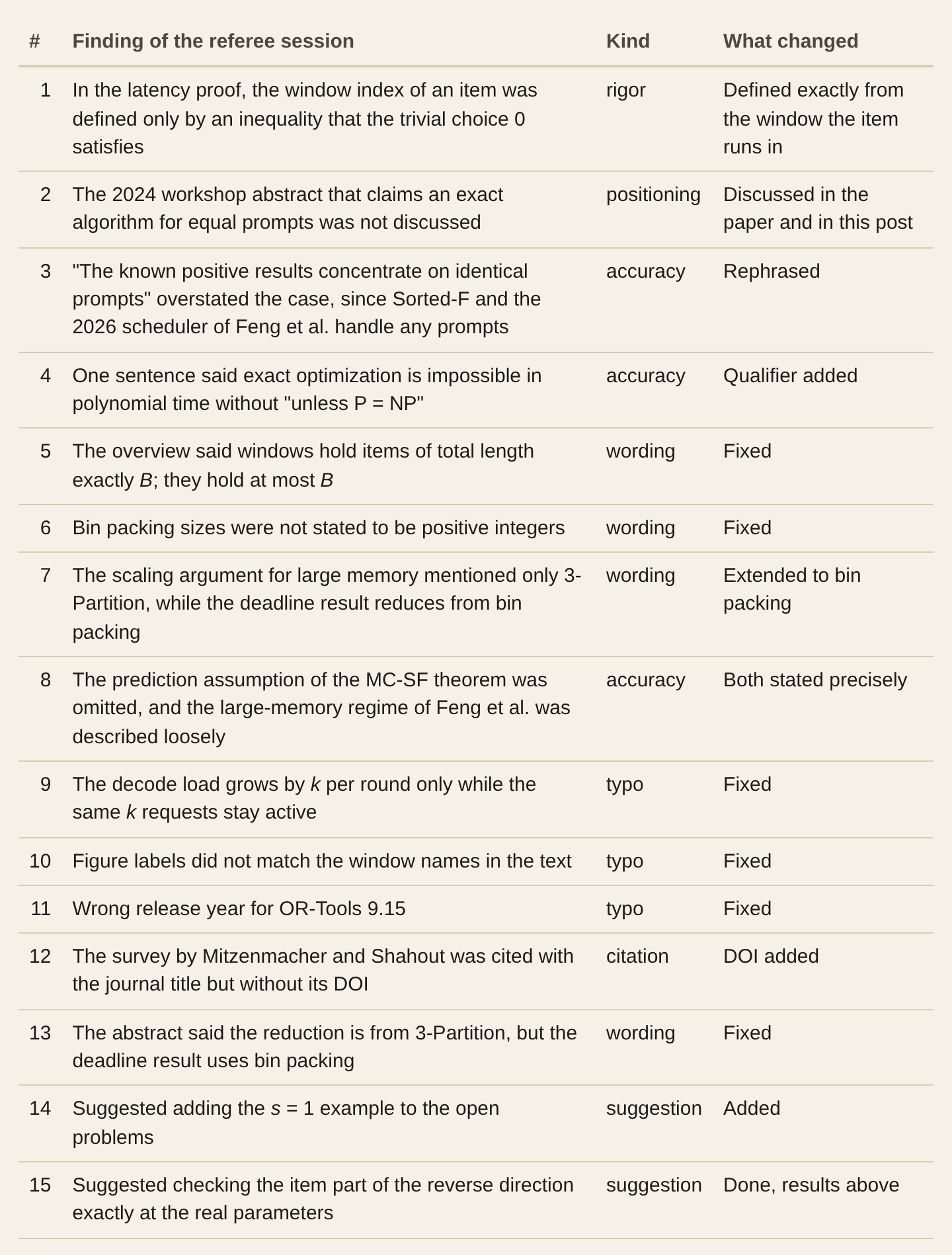
In the afternoon every claim was checked again. A third Claude session compared the external claims with their sources: the arXiv pages and PDFs of the papers, including the dates of the versions cited, the constants quoted and the exact text of the footnote; the source code of vLLM, SGLang and TensorRT-LLM; and bibliographic records for the classical papers.
It also recomputed the numbers of this work with its own code. It was cut short by a usage limit, and the last items were checked by the session that wrote the paper.
This round, and a last pass in the evening, found one real error, in the random study described below, and a number of statements that were less precise than their sources: how SGLang re-estimates its ratio after a retraction, which Llama release has the 128K context, which version of Jaillet et al. introduced MC-SF, and a few missing “unless P = NP” qualifiers. All of them were corrected in this post and in the paper.
A final pass then looked for what was missing rather than for what was wrong. The table lists every correction made after the referee round, and what that final pass added.

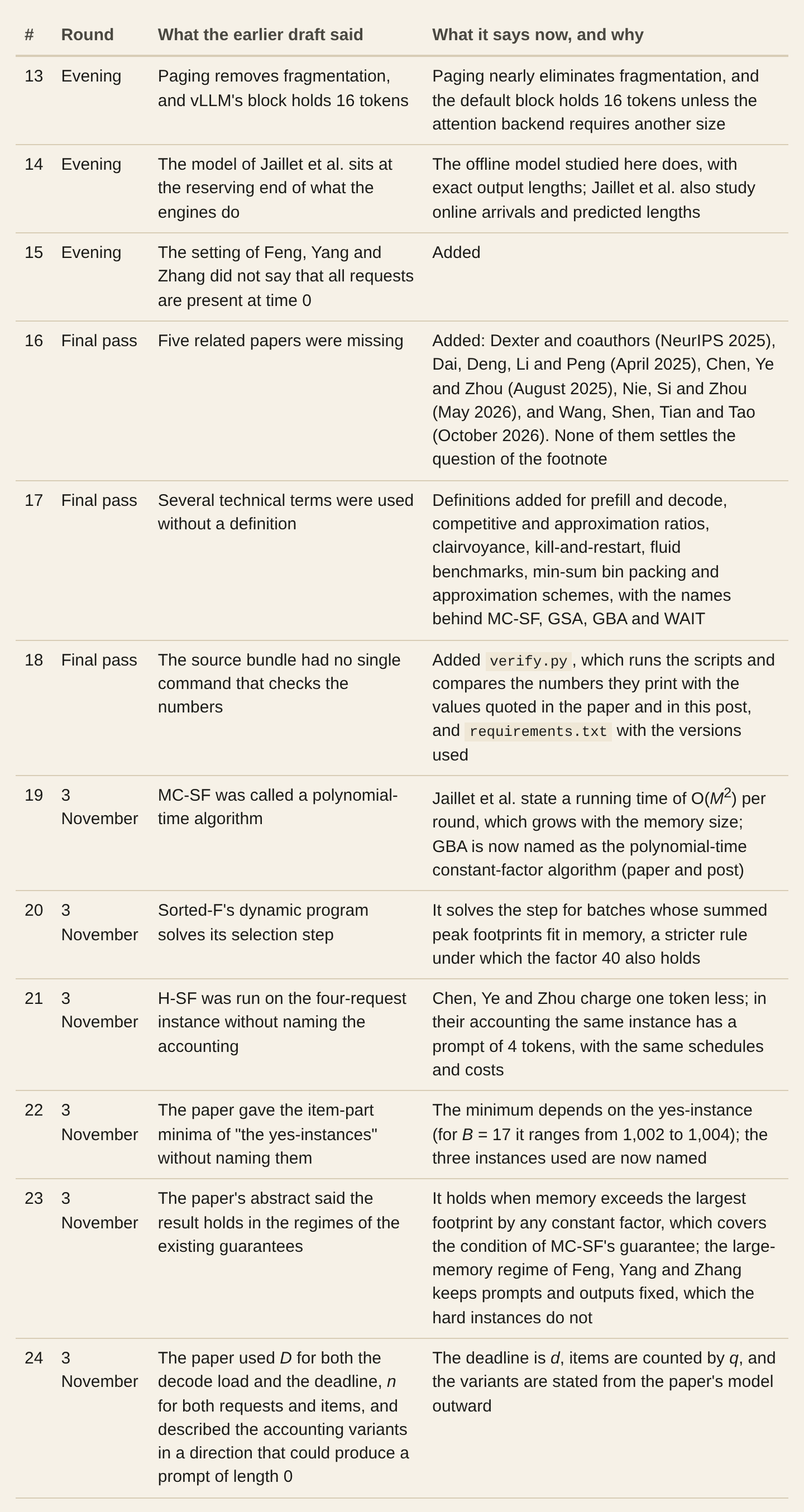

On the morning of 3 November, days before publication of this result, another intense Claude session, separate from all the others, reviewed the final version of the paper as a referee would. It had the paper and the scripts but was told not to trust the scripts, and it worked for about an hour.
It re-derived every proof, recomputed every number with its own code, including a fresh model of the 676 deadline instances that the paper then used and a fresh solver for the 1,000 random instances, checked each citation against its source, and searched for earlier proofs of the same result.
It found no error in the mathematics and no earlier proof. It did find statements that were looser than their sources, listed in the table above as the 3 November rows, and some notation and wording in the paper, which was fixed. One of its findings was itself wrong: it said that vLLM checks only the first chunk of a long prompt, but the code shows that the option named above makes the admission check cover the whole prompt, so the text stayed as it was.
Three more reviews, dated 3 November, came from the other agentic systems that we ran in parallel on our own machines, independently of the Claude sessions above: a referee report with its own scripts, a debate among three agents with distinct roles, a verifier, a skeptic and a computational arbiter, which had seen only the paper and not that report, and a list of corrections drawn from both.
None found a counterexample, and between them they reproduced with their own code the parameter table, the round-by-round example, the item costs of the reverse direction and the four-request example.
They did find five weak spots in how the argument and the checks were written. The most important, by the unanimous verdict of the debate, concerned the word “strongly”: the paper said only that the numbers of the constructed instances are polynomial in B and in the number of items, which is not enough when B is astronomically large, and the restriction described above, now spelled out in the paper, closes that gap.
The other four were a step in the proof of Lemma 4.2(a) compressed to the point of reading as false, a sentence in the proof of Corollary 7.1 that holds for the optimization problems but not for the deadline and target of the decision versions, a cap of five items in one cell of the test table that contradicted the stated rule of seven, and random seeds that the paper mentioned without giving them.
Each point was checked against the paper and the code before anything changed, and the 6 November rows of the corrections table list what changed. Another separate Claude session then checked the revised proofs, recounted the test table and the control predictions with its own code, and found no error, only a few places where the wording could be tighter, which were fixed.
The test table now has no cap and starts at B = 1, which one review suggested and another advised against, since bin packing with B = 1 is trivial. The scheduling instance is not: it is the smallest version of the construction, with three lanes, and the place where an off-by-one error in the arithmetic would show first.
What was not done: no human expert has reviewed the proof, and no full latency instance was solved exactly, since even the smallest has 9,372 requests and its wave schedule spans 131,124 rounds.
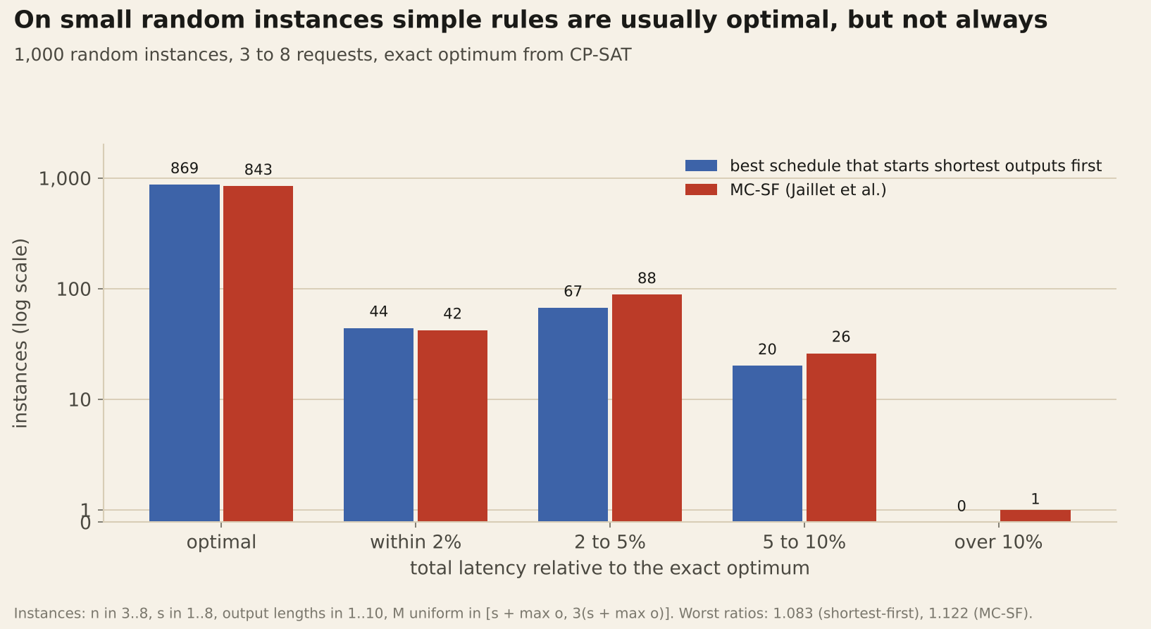
The random-instance study is a different kind of evidence. It does not test the proof; it asks how far simple rules are from optimal on ordinary small inputs. On 1,000 random instances with 3 to 8 requests, the best schedule that starts shorter requests first was optimal 869 times, 0.4% worse on average and never more than 8.3% worse.
MC-SF was optimal 843 times, 0.5% worse on average, and 12.2% worse in the worst case. These are corrected numbers. The first version of the study defined the schedules that start shorter requests first with constraints that were too weak when several requests had the same output length, which happens in most of these instances. It reported 955 instead of 869 and 6.3% instead of 8.3%, and it wrongly said that MC-SF’s worst instance had an optimal schedule of that kind.
MC-SF’s worst instance has eight requests, a one-token prompt, M = 15 and output lengths 8, 4, 9, 7, 7, 4, 5 and 7. The optimum is 90, the best schedule that starts shorter requests first costs 94, and MC-SF reaches 101, so it loses both on the order and on the timing of its greedy admissions.
The worst case for the order is small: s = 4, M = 13 and output lengths 1, 4, 4, 1 and 4. The optimum, 24, starts a length-4 request at time 0 next to one of the length-1 requests and delays the other length-1 request by one round; the best schedule that starts shorter requests first, which MC-SF also finds, costs 26.
What it means for a serving stack
If you run vLLM, SGLang or TensorRT-LLM in production, nothing in your scheduler is wrong because of this paper. The result is about exact optimization of admission decisions, which is out of reach in the worst case even in the friendliest version of the problem: one GPU, identical prompts, every output length known in advance, no arrivals after time zero.
Unless P = NP, no exact method runs in polynomial time on every instance, and that includes methods allowed to be pseudo-polynomial in the memory size. When a paper or a product claims an optimal scheduler for KV-cache admission, the useful question is which simplification makes optimality possible, or on which instances it is optimal.
Algorithms with constant-factor guarantees, like MC-SF and the geometric algorithms of Feng, Yang and Zhang, are the natural kind of result for this problem. GBA, the clairvoyant geometric algorithm, runs in polynomial time; for MC-SF, Jaillet et al. state a running time that grows with the square of the memory size at every round.
Unless P = NP, strong NP-hardness rules out a fully polynomial-time approximation scheme. Nobody knows whether a polynomial-time approximation scheme exists, one that reaches any fixed factor 1 + ε in polynomial time but may slow down sharply as ε shrinks, so for now a constant factor is the best kind of guarantee known to be achievable in polynomial time.
The hard instances have a recognizable shape: long common prompts, short outputs, and enough memory for many requests at once. The difficulty comes from the moments when the GPU is almost full and one more request fits only if the others are young.
Prefill-heavy workloads, with long prompts and short answers, are the ones closest to this regime, and the construction suggests where heuristics are most likely to lose against the optimum: at the boundary where admitting one more request depends on the age of the batch, not only on its size.
On small random instances, simple rules are close to optimal most of the time. The worst cases need structure, here synchronized waves of identical long requests, and production traffic is noisier than that, so the result says little about typical performance.
Comparing a scheduler with a hindsight optimum is a standard way to evaluate one in this literature, and computing that optimum is itself NP-hard, so exact comparisons are limited to small instances, or to larger ones that happen to be easy for a solver.
The natural integer program has one binary variable for every request and every possible start time, and one memory constraint per round. For the smallest hard instance above, even with the horizon cut to the 131,124 rounds of its wave schedule, that is 1,227,067,738 binary variables and 131,124 memory constraints.
On large traces, a reported gap to the optimum is in general measured against a relaxation, a bound or a heuristic solution, such as the hindsight shortest-first schedule H-SF, and it is worth checking which.
What the result does not cover
The theorem is about the offline problem in the model of Jaillet et al., and some features of real engines fall outside it. vLLM’s preemption keeps the generated tokens and rebuilds the cache, which the model would describe as a pause with a recomputation cost; the result says nothing about that variant, in which a request can leave memory and come back at the same point.
Chunked prefill, variable round times, block granularity and prefix sharing are not modeled. Online algorithms are measured by competitive ratio against the offline optimum, and a problem whose offline optimum is hard to compute can still have online algorithms with good ratios, as the constant-factor results above show.
What the theorem adds is that, unless P = NP, the yardstick those algorithms are measured against cannot be computed in polynomial time in general.
What is still open
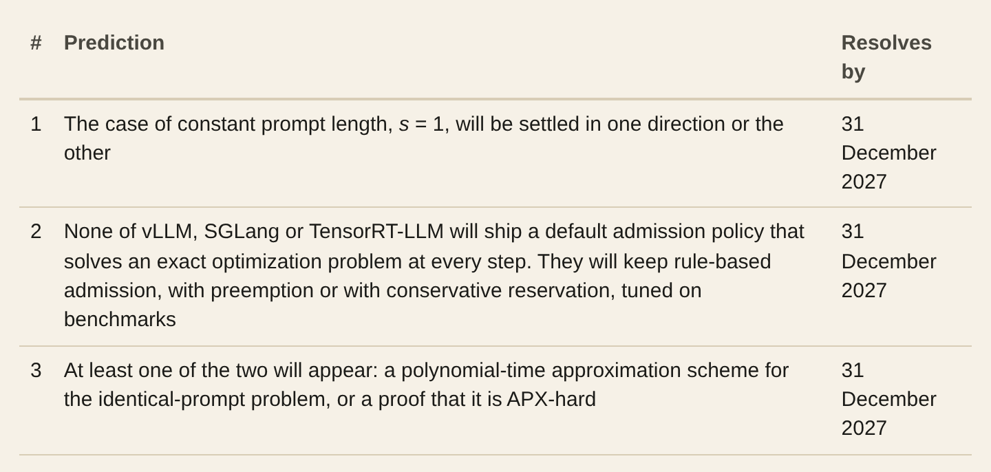
Short prompts. The proof needs prompts much longer than outputs, so that prompt memory caps the number of concurrent requests. When the prompt is a constant, say a single token, requests are almost free while they are young and no such cap exists. Whether the problem stays NP-hard with s = 1 is open, and the example with s = 1 above shows that the shortest-first structure fails there too.
Bounded concurrency. The hard instances need a number of lanes that grows with the instance, k = B + 2. In real deployments the number of requests that fit at once, roughly M/s, is often moderate. Is the problem polynomial, or at least pseudo-polynomial, when that number is a fixed constant? With one lane the problem is trivial, since requests run one at a time and shortest-first is optimal; for two lanes we do not know the answer.
Approximation. Constant-factor algorithms exist, and unless P = NP strong NP-hardness rules out an approximation scheme that is fully polynomial. The reduction in the paper loses only an additive L against a total of order kLN2, so it says nothing about constant-factor inapproximability. Strong NP-hardness alone does not settle the question either. With prompts of different lengths and one-token answers, the problem is exactly min-sum bin packing, with each round as a bin, and min-sum bin packing is strongly NP-hard yet has a polynomial-time approximation scheme, found by Leah Epstein, David Johnson and Asaf Levin. Whether the identical-prompt problem has such a scheme is open, and so is whether it is APX-hard, which would mean that for some constant c > 1, unless P = NP, no polynomial-time algorithm is always within a factor c of the optimum.
The conflicting claim. The December 2024 workshop abstract by Zijie Zhou and Jiashuo Jiang, presented at the NeurIPS 2024 workshop on Statistical Frontiers in LLMs and Foundation Models, assumes that all prompts have equal size, or sizes that grow with the output length, and that output lengths are predictable. It states that an algorithm doing O(n2) work per time period is optimal, describes the work as being in its early stages, and mentions two conjectures still to be validated. Only the abstract could be found, not the full text.
If that algorithm is meant for this model, it would run in pseudo-polynomial time, because an optimal schedule never has more rounds than the sum of the output lengths, and the result here implies it cannot be exact unless P = NP.
The most likely explanation is that the claim depended on those conjectures, or on a different model; their later paper with coauthors proves constant-factor guarantees instead. We have not had confirmation from the authors, and until then this point stays open.
How this was made
The request went in at 10:25, and Claude first asked which field and which format. Then it searched the recent literature for problems that were explicitly stated as open, read the candidates, and discarded several: the tight space bounds for streaming attention, for example, are the subject of active work by Indyk, Kapralov and coauthors, and the remaining gaps looked too deep for a single session.
The footnote of Wang, Ye and Zhou was crisp, recent, still open in a version posted five weeks earlier, and squarely in the area of this newsletter.
Before trying to prove anything, it wrote an exact solver for small instances and ran experiments. In a first batch of 300 random instances, some had no optimal schedule that starts shorter requests first: 7 by the count printed at the time, 29 after the correction described above.
That was the hint that the problem has real combinatorial structure, and the search for a reduction began. The lane view came from looking at what a large common prompt does to the memory constraint; the frames, waves and windows came from asking how to make the last lane open for a controlled number of rounds; the tail came from noticing that without it the items would simply go first.
The paper was written in LaTeX, with figures generated from the same code that checks the constructions. A second, independent Claude session then reviewed it as a referee for about half an hour, and its corrections went into the first complete version, twelve pages long, finished at 11:47.
In the afternoon, at our request, every claim in the paper and in this post was checked again against its source, and the paper was expanded with a worked example, a table of parameters and a few remarks that make the argument easier to follow.
A final pass looked for what was missing: five related papers, the definitions a reader outside the field needs, and a script that checks the computed numbers in the paper and in this post against the output of the code.
On 6 November, after the three reviews described above, the paper was revised once more, mainly to spell out the strong NP-hardness argument and to extend the solver check. In the afternoon of the same day it gained a second author and an appendix that prints the code. The version attached here has thirty-two pages.
Several systems worked on this, and none of them saw another’s work unless we passed it on. This is who did what.
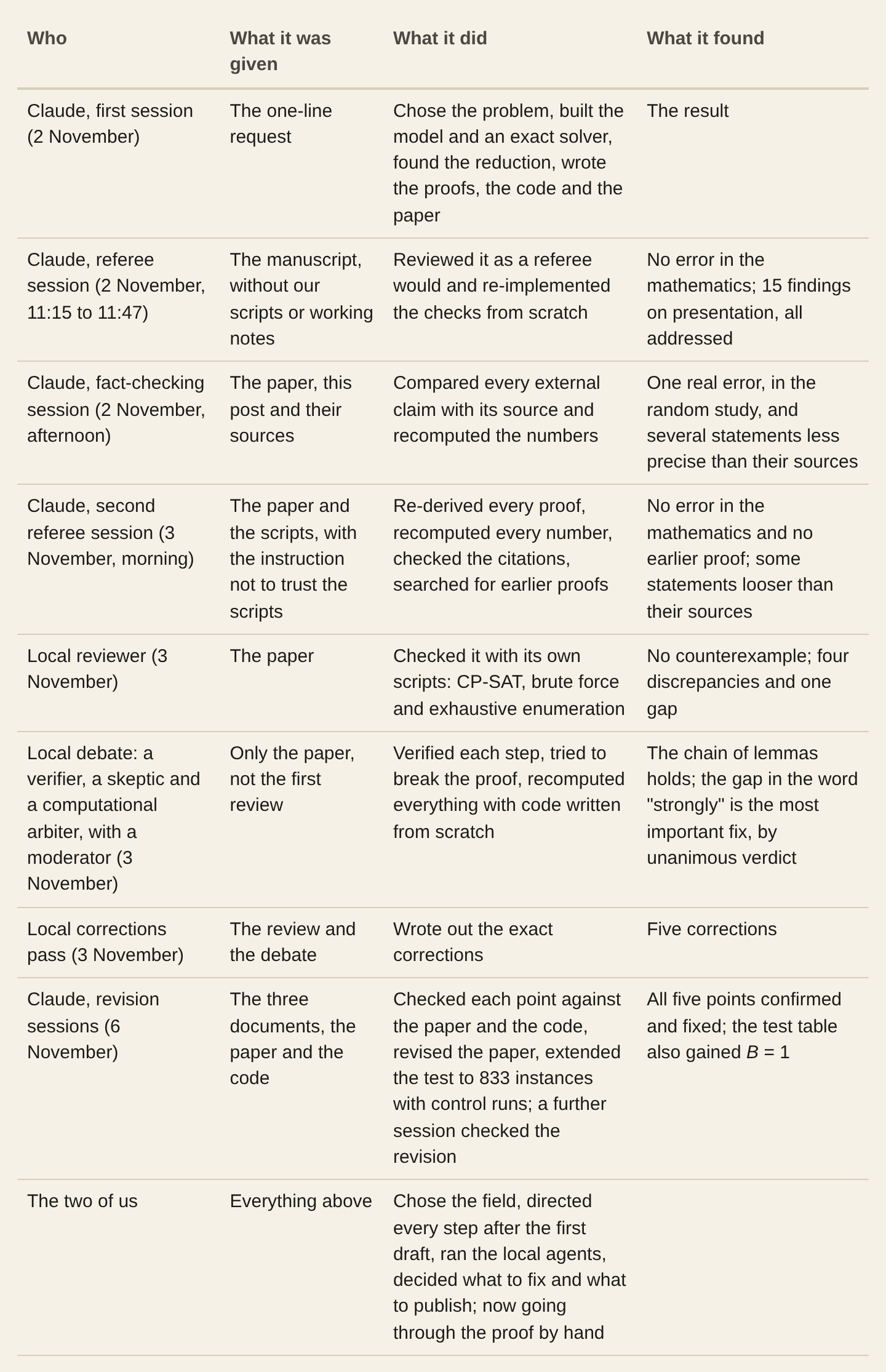
The tools were ordinary: Python, OR-Tools CP-SAT 9.15 for exact solving, matplotlib for the figures, pdflatex for the paper. Claude’s sessions ran on a small cloud container with two CPU cores and no GPU; the other agents ran on our own machines.
And this is the order in which it happened.
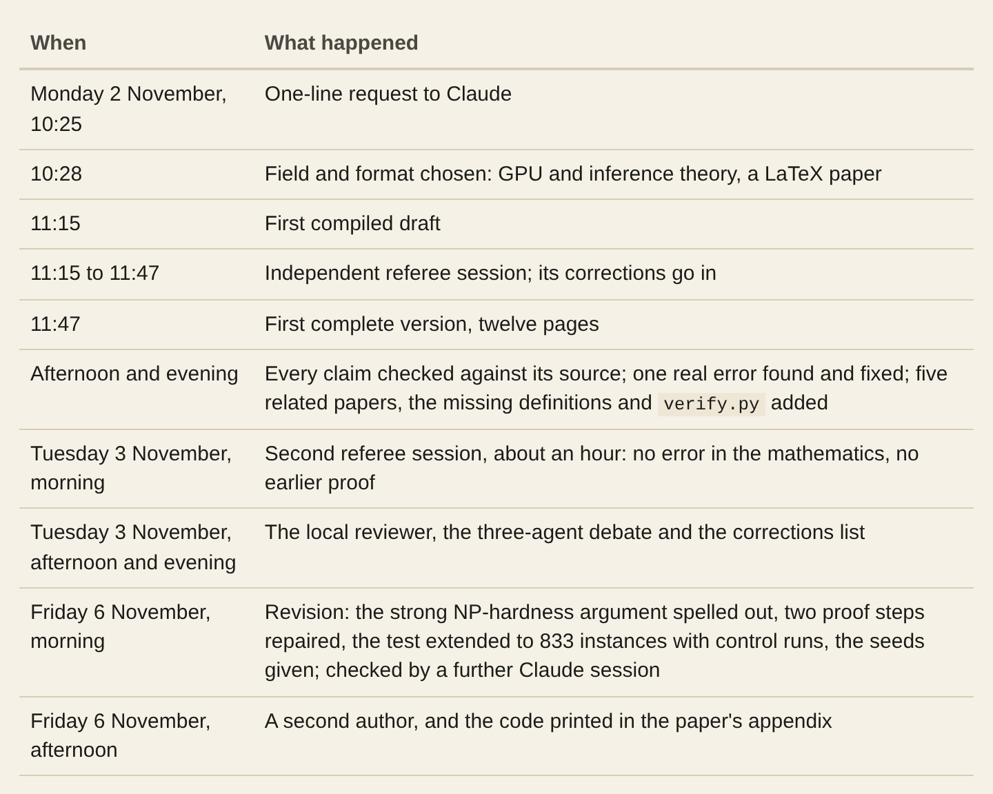
The proof is Claude’s. The decision to publish it, with this account of how it was made, is ours, and so is the responsibility for any mistake that the automated reviews missed. If you find one, please tell us.
Reproducing every number
The source bundle of the paper has a folder named anc with the scripts. They need Python 3 and OR-Tools 9.15, and matplotlib for the figures; requirements.txt pins the versions used. Every random instance is generated from a fixed seed, given in the paper and checked by verify.py, so the numbers in this post come out exactly.
The script verify.py runs the others and checks the numbers they compute against the values quoted in the paper and in this post, printing PASS or FAIL for each. The subfolder anc/independent holds the code of the independent review, unchanged except for one option, added on 6 November, that extends its deadline check to the current test table.
The exact solver behind most of these checks fits on one screen. It has one yes-or-no variable for every request and every possible start time, one memory constraint per round, and it minimizes the sum of completion times.
This is the function from kvmodel.py, unchanged; Appendix B of the paper prints it together with the other main scripts.
def cpsat_min_tel(lengths, s, M, order=None, time_limit=120, workers=2):
    """Exact minimum TEL by a time-indexed CP-SAT model with horizon sum(lengths).
    The horizon is safe: an optimal schedule never leaves a round empty before its last
    completion (otherwise every later request could be moved one round earlier).
    order: optional list of pairs (a, b) imposing start[a] <= start[b]."""
    n = len(lengths)
    H = sum(lengths)
    m = cp_model.CpModel()
    x = {}
    for i, o in enumerate(lengths):
        for p in range(H - o + 1):
            x[i, p] = m.NewBoolVar("")
        m.AddExactlyOne(x[i, p] for p in range(H - o + 1))
    start = [sum(p * x[i, p] for p in range(H - o + 1)) for i, o in enumerate(lengths)]
    for t in range(1, H + 1):
        terms = [(s + t - p) * x[i, p] for i, o in enumerate(lengths)
                 for p in range(max(0, t - o), min(t - 1, H - o) + 1)]
        if terms:
            m.Add(sum(terms) <= M)
    for a, b in (order or []):
        m.Add(start[a] <= start[b])
    m.Minimize(sum(start) + sum(lengths))
    solver = cp_model.CpSolver()
    solver.parameters.max_time_in_seconds = time_limit
    solver.parameters.num_workers = workers
    st = solver.Solve(m)
    if st != cp_model.OPTIMAL:
        raise RuntimeError("not solved to optimality")
    return int(round(solver.ObjectiveValue())), [int(solver.Value(v)) for v in start]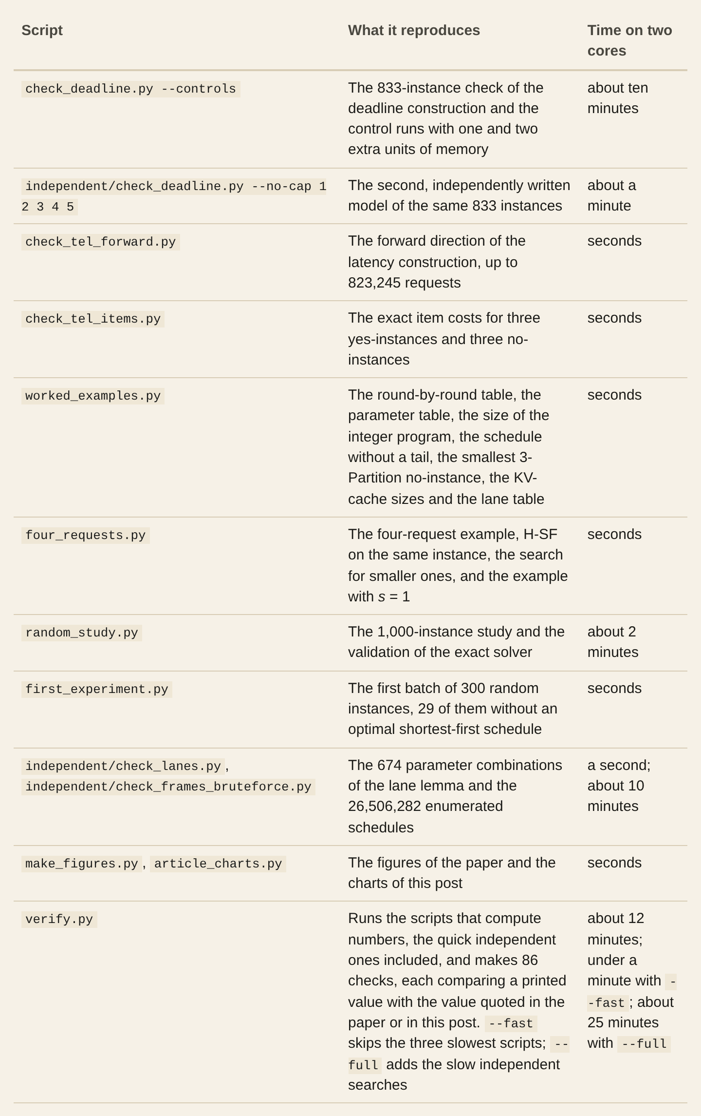
Where we might be wrong
The proof could contain an error that the automated reviews missed. The most delicate step is the claim that a schedule meeting the target must keep the first m + 1 waves exactly aligned; it rests on the chain property of frames and on the size of the tail.
The exhaustive enumerations and the solver checks cover the lemmas behind it on small instances, but small instances are not a proof. Three further reviews in November found no counterexample, but they did find a real gap in how the paper justified the word “strongly”, now closed. That is a reason for more confidence, not for certainty.
The model could differ from what Wang, Ye and Zhou had in mind. Their fifth version specifies memory si + j for the j-th token, no preemption, total latency as the objective, and all requests at time zero in the offline setting.
The proof matches that text. It also survives the obvious variations: charging s + j − 1 instead of s + j, or processing the prompt in its own round before the first token, both reduce to the same model after shifting the parameters.
The question might already have been answered somewhere we did not look. A last search for related work found five papers that the first version had missed, and a search on 6 November found one more, posted on 3 November; none of them settles the footnote, but another paper could exist.
The Zhou and Jiang abstract could describe a model where their algorithm is exact for good reasons. If so, the two results are about different problems, and we will say so.
The practical reading could be wrong in the other direction. NP-hardness is a statement about the worst case. It is possible that the instances that matter in production have structure that makes them easy, and the random study above is consistent with that.
Three predictions
The paper, Minimizing Latency under a KV-Cache Budget Is Strongly NP-Hard, Even with Identical Prompts, is attached below. If you work on scheduling theory and want to check the argument, the main proof takes a few pages, starting with the lane lemma in Section 3; its Appendix B prints the code, and the scripts in the source bundle reproduce every number in this post that comes from a computation. Tell us what you find, in the comments or by replying to this email.
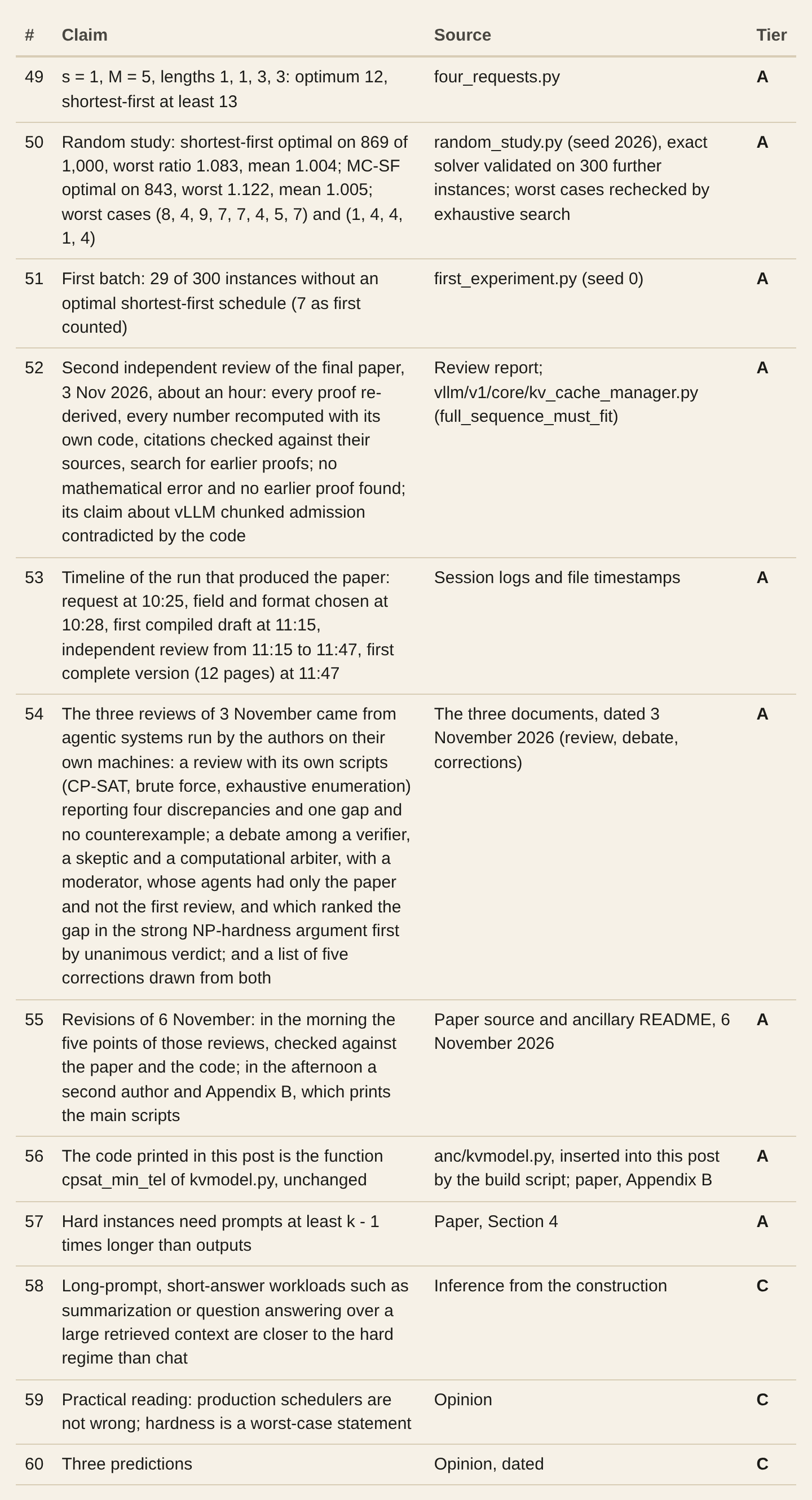
Verification dossier
Tier A: checked against the primary source or reproduced by code in this work. Tier B: checked against an authoritative secondary source. Tier C: inference or estimate, stated as such in the text. Tier D: not verified.

References
P. Jaillet, J. Jiang, K. Mellou, M. Molinaro, C. Podimata, Z. Zhou. Online Scheduling for LLM Inference with KV Cache Constraints. arXiv:2502.07115, v1 February 2025, v5 January 2026. arxiv.org/abs/2502.07115
M. Wang, Y. Ye, Z. Zhou. LLM Serving Optimization with Variable Prefill and Decode Lengths. arXiv:2508.06133, v1 August 2025, v5 September 2026. arxiv.org/abs/2508.06133
Y. Feng, Z. Yang, Y. Zhang. Competitive Non-Clairvoyant KV-Cache Scheduling for LLM Inference. arXiv:2601.22996, January 2026. arxiv.org/abs/2601.22996
Y. Feng, S. Liu, Z. Yang, Y. Zhang. General Non-Clairvoyant KV-Cache Scheduling via Regime-Aware Routing. arXiv:2607.09248, July 2026. arxiv.org/abs/2607.09248
I. D’Ambrosio. A Tight Linear Deterministic Competitive Ratio for Fully Online KV-Cache Scheduling. arXiv:2608.16944, August 2026. arxiv.org/abs/2608.16944
R. Ao, G. Luo, D. Simchi-Levi, X. Wang. Optimizing LLM Inference: Fluid-Guided Online Scheduling with Memory Constraints. arXiv:2504.11320, v1 April 2025, v4 June 2026. arxiv.org/abs/2504.11320
M. Mitzenmacher, R. Shahout. Queueing, Predictions, and Large Language Models: Challenges and Open Problems. Stochastic Systems 15(3):195-219, 2025, doi:10.1287/stsy.2025.0106. Preprint titled Queueing, Predictions, and LLMs: Challenges and Open Problems, arXiv:2503.07545, March 2025. arxiv.org/abs/2503.07545
Z. Zhou, J. Jiang. Scheduling in LLM Inference with Blowed-up Memory Constraints. Poster, NeurIPS 2024 Workshop on Statistical Frontiers in LLMs and Foundation Models, 14 December 2024. neurips.cc/virtual/2024/105592
Z. Chen, Y. Ye, Z. Zhou. Adaptively Robust LLM Inference Optimization under Prediction Uncertainty. arXiv:2508.14544, v1 August 2025, v2 September 2025. arxiv.org/abs/2508.14544
G. Dexter, S. Tang, A. Fatahi Baarzi, Q. Song, T. Dharamsi, A. Gupta. LLM Query Scheduling with Prefix Reuse and Latency Constraints. NeurIPS 2025. arXiv:2502.04677, v1 February 2025, v3 January 2026. arxiv.org/abs/2502.04677
X. Wang, H. Shen, H. Tian, Y. Tao. Approximation Algorithms for Dual-Memory Request Scheduling in Disaggregated LLM Inference. arXiv:2610.15579, October 2026. arxiv.org/abs/2610.15579
J. G. Dai, T. Deng, Y. Li, T. Peng. Throughput-Optimal Scheduling Algorithms for LLM Inference and AI Agents. arXiv:2504.07347, v1 April 2025, v3 May 2026. arxiv.org/abs/2504.07347
C. Nie, N. Si, Z. Zhou. A Queueing-Theoretic Framework for Stability Analysis of LLM Inference with KV Cache Memory Constraints. arXiv:2605.04595, May 2026. arxiv.org/abs/2605.04595
Z. Li, S. Wang, N. Si. Asymptotic Optimality of cμ-Rule for LLM Inference Scheduling under Memory Constraint. arXiv:2611.04807, 3 November 2026. arxiv.org/abs/2611.04807
A. Agrawal, N. Kedia, J. Mohan, A. Panwar, N. Kwatra, B. Gulavani, R. Ramjee, A. Tumanov. Vidur: A Large-Scale Simulation Framework For LLM Inference. MLSys 2024. arXiv:2405.05465. arxiv.org/abs/2405.05465
G.-I. Yu, J. S. Jeong, G.-W. Kim, S. Kim, B.-G. Chun. Orca: A Distributed Serving System for Transformer-Based Generative Models. OSDI 2022, pages 521-538. usenix.org/conference/osdi22/presentation/yu
W. Kwon, Z. Li, S. Zhuang, Y. Sheng, L. Zheng, C. H. Yu, J. E. Gonzalez, H. Zhang, I. Stoica. Efficient Memory Management for Large Language Model Serving with PagedAttention. SOSP 2023, pages 611-626, doi:10.1145/3600006.3613165. arxiv.org/abs/2309.06180
Llama Team, AI @ Meta. The Llama 3 Herd of Models. arXiv:2407.21783, 2024. arxiv.org/abs/2407.21783
Meta AI. Introducing Llama 3.1: Our most capable models to date. 23 July 2024. ai.meta.com/blog/meta-llama-3-1/
vLLM documentation. Optimization and Tuning, section on preemption. docs.vllm.ai/en/latest/configuration/optimization/
vLLM source code, main branch, retrieved 2 November 2026 and checked again on 3 November 2026:
vllm/config/scheduler.py,vllm/config/cache.py,vllm/platforms/interface.py,vllm/v1/core/sched/scheduler.py,vllm/v1/core/kv_cache_manager.py; for the old warning,vllm/core/scheduler.pyat release v0.6.0. github.com/vllm-project/vllmSGLang source code, main branch, retrieved 2 November 2026 and checked again on 3 November 2026: in
python/sglang/srt/, the filesmanagers/schedule_policy.py,managers/schedule_batch.py,managers/scheduler.py,managers/scheduler_components/new_token_ratio_tracker.py,mem_cache/prefill_budget.py,environ.pyandarg_groups/fields/schedule.py. github.com/sgl-project/sglangSGLang documentation. Hyperparameter Tuning. docs.sglang.io/advanced_features/hyperparameter_tuning.html
NVIDIA TensorRT-LLM, main branch, retrieved 2 November 2026 and checked again on 3 November 2026:
tensorrt_llm/llmapi/llm_args.py, and the performance tuning guide Useful Runtime Options,docs/source/legacy/performance/performance-tuning-guide/useful-runtime-flags.md. github.com/NVIDIA/TensorRT-LLMM. R. Garey, D. S. Johnson. Complexity Results for Multiprocessor Scheduling under Resource Constraints. SIAM Journal on Computing 4(4):397-411, 1975, doi:10.1137/0204035. See also Computers and Intractability, W. H. Freeman, 1979.
M. R. Garey, D. S. Johnson. “Strong” NP-Completeness Results: Motivation, Examples, and Implications. Journal of the ACM 25(3):499-508, 1978, doi:10.1145/322077.322090.
J. Bruno, E. G. Coffman, R. Sethi. Scheduling Independent Tasks to Reduce Mean Finishing Time. Communications of the ACM 17(7):382-387, 1974, doi:10.1145/361011.361064.
L. Epstein, D. S. Johnson, A. Levin. Min-Sum Bin Packing. Journal of Combinatorial Optimization 36(2):508-531, 2018, doi:10.1007/s10878-018-0310-x.
J. Y. Chen, Y. Feng, P. Indyk, M. Kapralov, E. Kochetkova, B. Prokhorov. Towards Tight Bounds for Streaming Attention. arXiv:2606.07205, June 2026. arxiv.org/abs/2606.07205
Argonne National Laboratory. Argonne at NeurIPS 2024, event listing with the date of the workshop on Statistical Frontiers in LLMs and Foundation Models. anl.gov/mcs/article/argonne-at-neurips-2024
L. Perron, F. Didier. CP-SAT, Google OR-Tools 9.15 (released January 2026). developers.google.com/optimization
L. Bradanini, L. Tettamanti. Minimizing Latency under a KV-Cache Budget Is Strongly NP-Hard, Even with Identical Prompts. Preprint, November 2026, attached to this post.