



Intro
Most of the pieces I’ve written here end with a number. A critical batch size, a cost per million tokens, a speedup from speculation. Somewhere down the chain, almost every one of those numbers rests on somebody’s benchmark, and a few of them are benchmark results I quoted directly.
For a long time I treated those results the way I treat a datasheet: as a property of the hardware and the engine being measured.
That was too generous. A benchmark of an LLM server is produced by three programs together: the server, the load generator that decides when each request leaves and what it contains, and the arithmetic that turns a few hundred thousand timestamps into one row of a table. The public argument is almost entirely about the first program.
When I went looking for where the numbers actually move, most of the movement I could find came from the other two.
So I did two things. I read the timing code of the tools behind many of the numbers people quote today: vLLM’s bench serve, SGLang’s serving benchmark, the client behind SemiAnalysis’s InferenceX, NVIDIA’s AIPerf, GuideLLM, LLMPerf and MLPerf’s LoadGen, all at their October 2026 heads. Then I built a small simulator of a continuous batching server and pointed each of those methods at it.
A simulated server answers identically every time, which no GPU does, so when two numbers differ, the method is the only thing left to blame.
Some of what follows is old news to anyone who has load-tested a web service, and part of the argument about metrics was made carefully in 2024 by the authors of Etalon. The client-side effects I have not seen measured before.
The short version is that in a fixed-concurrency run the printed p99 time to first token can come entirely from the first wave of requests, that a concurrency cap on the client hides exactly the queue it creates, that the peak of a concurrency sweep sits on the edge of a cliff the sweep cannot see, and that a token is not the same unit in two different tools, or for two different models.
The instrument
The simulator is about 350 lines of Python, and the core of it is in the appendix. The server follows the shape of vLLM’s V1 scheduler. Each engine step has a token budget.
Running requests are served first, one token for those decoding and a chunk of prompt for those still in prefill, then waiting requests are admitted in arrival order while the budget, the sequence cap and the KV pool allow.
KV cache is allocated in 16-token blocks as tokens are computed, and when the pool runs out the most recently admitted request is preempted and later recomputed from scratch. A request is just a count of computed tokens chasing a target, which covers prefill, decode and recompute with a single rule. That is also how vLLM’s V1 scheduler thinks about it.
I set the budget to 8,192 tokens and the sequence cap to 1,024 because those are the defaults vLLM picks for its API server on an H100-class GPU; they are in vllm/engine/arg_utils.py, keyed on device memory.
The model has the shape of Llama 3.1 8B in BF16: 32 layers, 8 KV heads of dimension 128, so 128 KiB of KV per token, and 15.0 GB of weights streamed per step once the embedding table is excluded.
Step time is a roofline: a fixed 1 ms of overhead for scheduling, launch and sampling, plus the larger of compute time at 75% of the 989.4 TFLOP/s dense BF16 peak and memory time at 85% of 3.35 TB/s. The KV pool holds 430,000 tokens.
With those numbers, a batch-one decode step takes 6.3 ms, which is 158 tokens per second for a single user. A 1,024-token prefill takes 20.6 ms. A full 8,192-token chunk of prefill takes 158 ms, about 52,000 tokens per second. They are plausible for this model on this GPU, and later I rerun four of the main effects under eleven versions of the model to see how much they depend on those values.
It is also not the first simulator of an LLM server. Vidur, presented at MLSys 2024, combines profiles of real operators on real GPUs with predictive models, estimates latency with less than 9% error, and comes with a search tool for deployment configurations. Mine is much cruder on purpose.
The subject here is the client and the arithmetic, and for that a server whose every constant fits in one table is easier to reason about than a faithful one.
What the simulator cannot do is tell you what an H100 will measure. There is no network, no HTTP server, no SSE framing, no tokenizer in the loop, no kernel launch jitter, no speculative decoding. The absolute numbers belong to a model of a GPU, and I will say so every time I use one.
What it can do is show mechanisms, their direction and their rough size, with every run reproducible from a seed. When I write that a method moves a number by twenty times, I mean it does so in this model, and I will describe the mechanism so you can decide whether your system has it.
Where the clock starts
The first thing I did was to write down, for each tool, three facts that are rarely printed next to its results: when the clock starts, what counts as the first token, and what the per-token number divides by what.
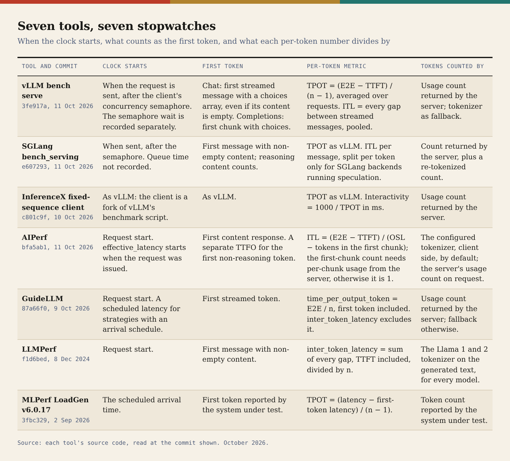
Some of the differences in that table are about edge cases. vLLM’s chat client stamps the first token on the first streamed message that carries a choices array, even when its content is empty, while SGLang and LLMPerf wait for non-empty content.
On vLLM’s own server the two agree, because the empty role message and the first token leave in the same iteration of the response loop. On a server that acknowledged a request with an empty message before prefill, they would not.
Other differences are not edge cases at all.
In vLLM, TPOT is the time between the first and the last token divided by the number of gaps between them, averaged over requests, and ITL is every single gap between two streamed messages, pooled across the run.
In GuideLLM,
time_per_output_tokenis the whole request duration divided by the number of tokens, so the wait for the first token is spread over the answer, and it is GuideLLM’sinter_token_latencythat matches vLLM’s TPOT.LLMPerf sums every gap including the time to first token and divides by a token count taken with the Llama 2 tokenizer, whatever model produced the text.
AIPerf, when the server reports usage per chunk, divides by the output length minus however many tokens arrived in the first chunk, because some servers bundle several tokens there.
MLPerf’s LoadGen starts every clock at the moment a request was scheduled, not the moment it was sent.
None of these is wrong. They answer different questions. The trouble is that they share three or four names, and the numbers they produce are printed with two decimal places and pasted into comparison tables next to each other.
To see how far apart they land, I took one simulated run and computed every definition on it. The run is what you get from vllm bench serve with its default lengths, 1,024-token prompts and 128-token outputs, and 64 users.
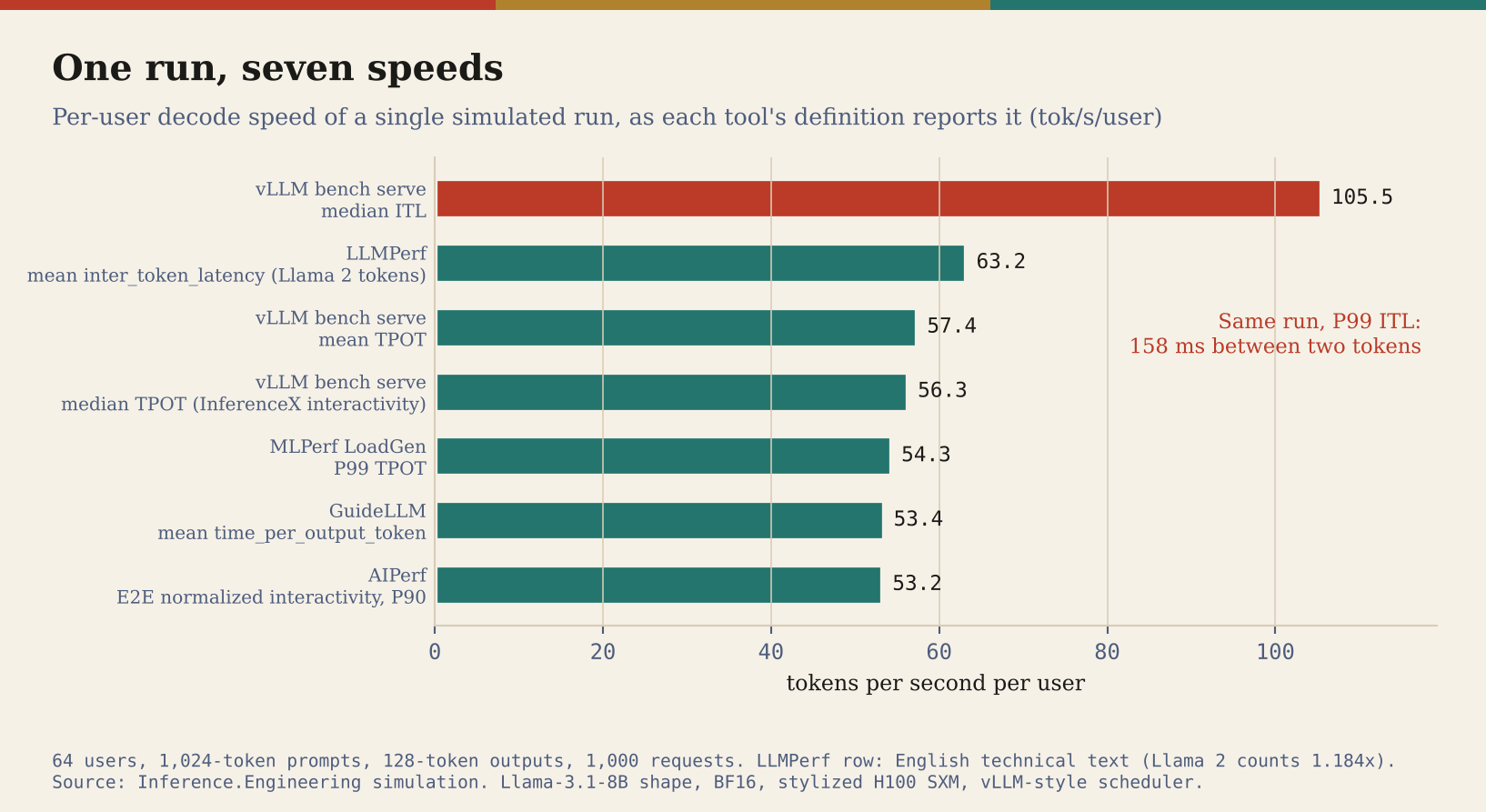
From the same run, the per-user speed comes out anywhere between 53.2 and 105.5 tokens per second depending on which definition you apply. The gap is not noise. The median ITL of 9.5 ms is the pace of a pure decode step, which is what most steps are.
The mean TPOT of 17.4 ms is slower because about one gap in seventeen lands on a step where somebody else’s prompt is being prefilled, and those steps take up to 158 ms; 5.9% of all gaps in this run are longer than 100 ms. GuideLLM’s and AIPerf’s numbers are slower still because they fold in the wait for the first token.
LLMPerf’s comes out faster than TPOT because it counts 18% more tokens than the model produced, for reasons I come back to below.
Each of these is a reasonable thing to report. The median ITL is how a stream feels most of the time, the p99 ITL is the stutter you notice, TPOT is the average pace once the answer has started, and duration divided by tokens is the pace including the wait.
What is not reasonable is a table where the left column came from one tool and the right column from another, and both are labeled time per output token.
The complaint about the metrics themselves is not new.
In 2024 the authors of Etalon, the group behind the Sarathi-Serve scheduler and the Vidur simulator, showed that TPOT can hide intermittent stalls inside an average, that normalized latency hides the time a request waits to be scheduled, and that a tail percentile of the gaps between tokens says little about how long and how often a request stalls; they proposed a deadline-based fluidity index instead.
The 158 ms gaps in my run are the kind of stall Sarathi-Serve was designed to bound, where decodes that share a step with a large chunk of somebody else’s prompt wait for the whole chunk.
What I had not seen written down is the version of the problem that lives in the tools, where the same few names are bound to different formulas in the scripts people run every day and the results are pasted side by side.
The first wave
Many of the serving numbers published today come from fixed-concurrency runs. In vLLM’s client that is --max-concurrency N with the request rate left at its default, which is infinite; the help text says that with an infinite rate every request is sent at time zero.
The semaphore then lets N of them through, and every time one finishes, the next one goes.
SemiAnalysis’s InferenceX uses exactly this setup in its fixed-sequence runs: the single-node fixed-sequence client in its repository, at commit c801c9f, sets the number of prompts to ten times the concurrency, the rate to infinity, the warmups to twice the concurrency, and computes percentiles over every request.
The warmup warms the engine, not the queue. After the warmup requests finish, the server is idle again, and the measured run starts the same way the warmup did, with N requests arriving at an empty server in the same instant.
The engine prefills them in chunks, eight 1k prompts per 8,192-token step, and the last request of the wave waits for all of the others. Its time to first token is roughly N times the mean prompt length divided by the prefill rate, which at 64 users is 64 × 921.5 / 51,800, about 1.14 s.
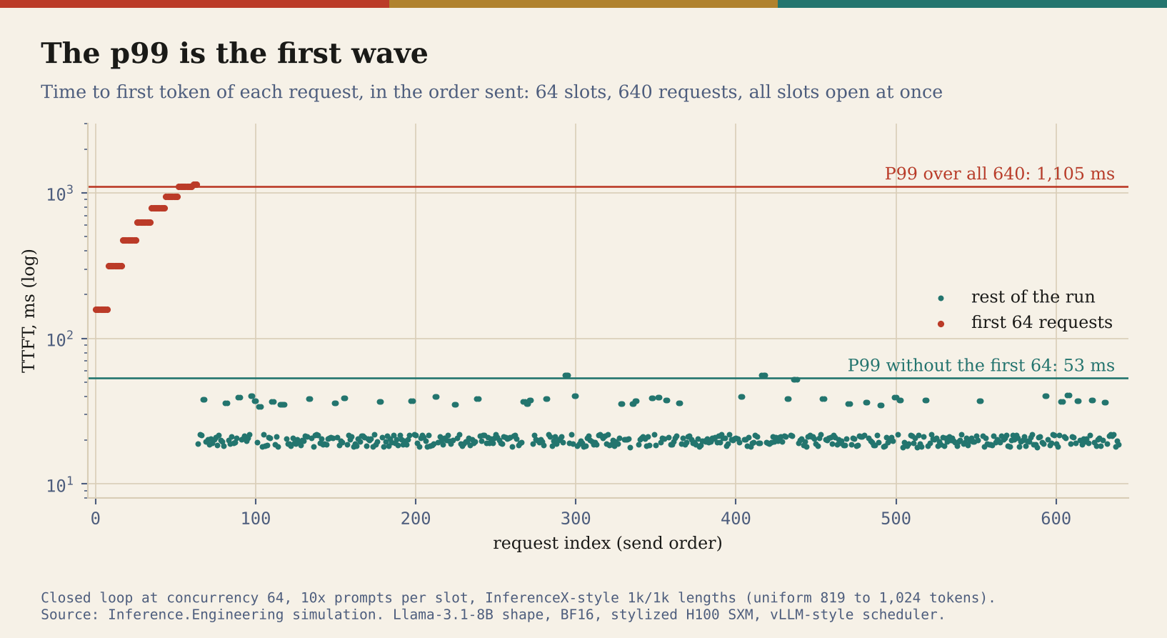
In a run of 640 requests at 64 slots with InferenceX’s 1k/1k lengths, the p99 time to first token over the whole run is 1,105 ms. Without the first 64 requests it is 53 ms. The median is about 20 ms either way.
The first wave is 10% of the sample and the p99 looks at the top 1%, so the p99 sits entirely inside the wave. It does not describe the server under load at all; it describes how long the server takes to work through a thundering herd, and it grows linearly with the concurrency.
At 16 slots the same comparison gives 284 ms against 37 ms, at 256 slots 4,265 ms against 105 ms, averaged over three seeds. Collecting twenty or fifty times the concurrency instead of ten does not fix it, because the wave is still more than 1% of the sample, and at fifty times the p99 is still 631 ms.
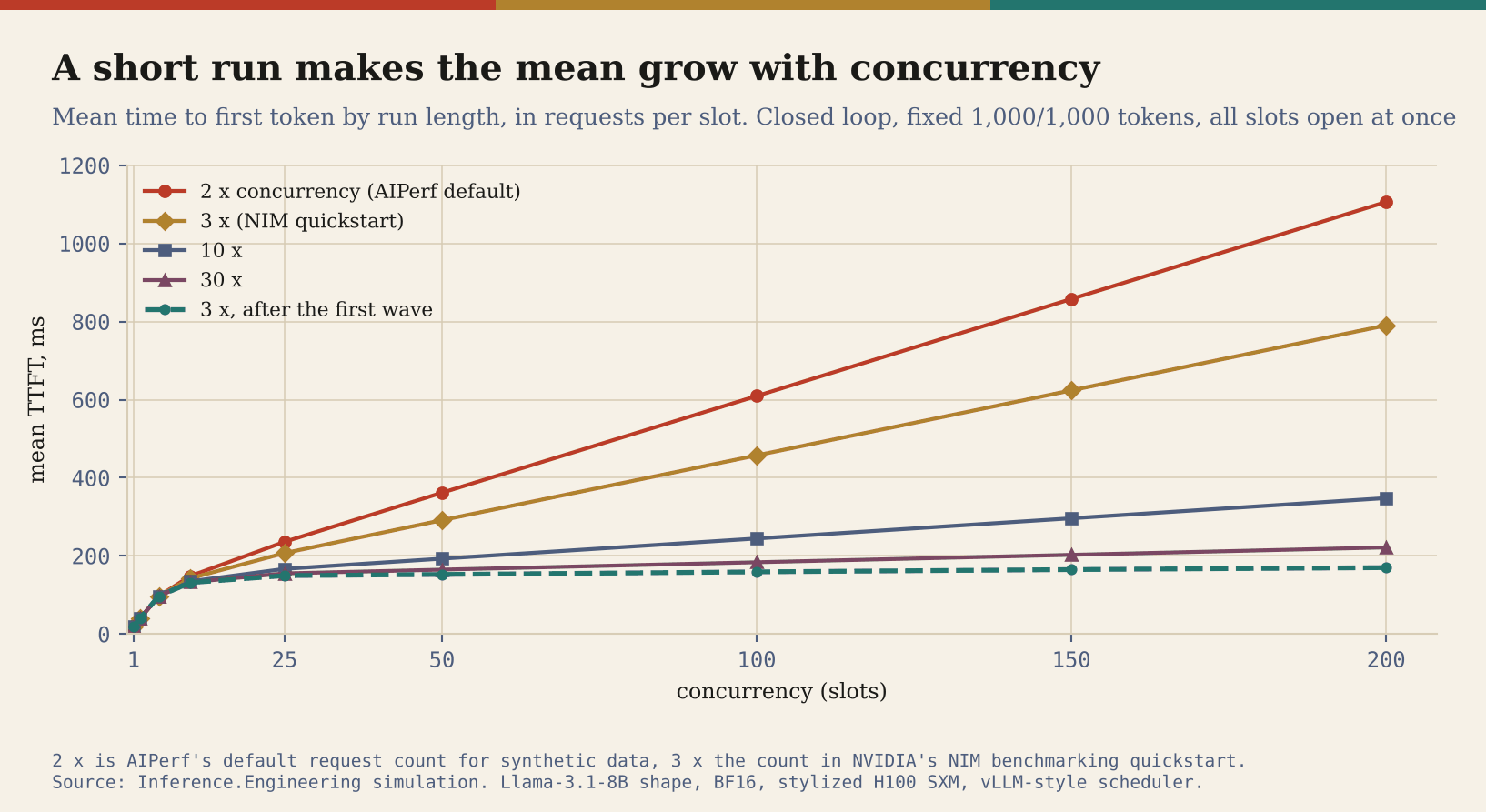
AIPerf, the NVIDIA tool that the NIM benchmarking guide is built around, also opens every slot at once by default, and it collects fewer requests. Its documentation says that for synthetic data the default number of requests is max(10, concurrency * 2), so at any concurrency above five a default run is two waves, and the quickstart in the NIM guide sets the request count to three times the concurrency, which it describes as enough for a stable measurement.
AIPerf has a remedy built in, --concurrency-ramp-duration, which raises the concurrency from one to the target over a given number of seconds. It is not the default.
With three times the concurrency a third of the samples belong to the wave, and with twice the concurrency half of them, so it is no longer only the p99 that comes from it. I replayed both recipes on the simulator with fixed lengths of 1,000 tokens in and 1,000 out.
At three times the concurrency, the mean time to first token grows from 207 ms at 25 users to 790 ms at 200. After the first wave it stays between 149 and 170 ms over the same range.
At twice the concurrency, the mean at 200 users is 1,106 ms, and even the median is twice what it is at three times, 317 ms against 158, because it now sits at the edge of the wave. A column of mean times to first token measured this way grows with concurrency almost entirely because of how the run starts.
Running vllm bench serve with no rate and no concurrency flag at all gives the extreme case, with all 1,000 default prompts arriving together. In the model, the median time to first token of that run is 12.9 s and the p99 is 25.1 s, with 47 preemptions along the way. It is a measurement of 1,000 users arriving in the same instant.
The wave has a second edge at the other end. Throughput is usually computed as total output tokens divided by the duration of the whole run, and the whole run includes the start, where the server is busy prefilling instead of decoding, and the drain, where the last few requests finish with the batch emptying around them.
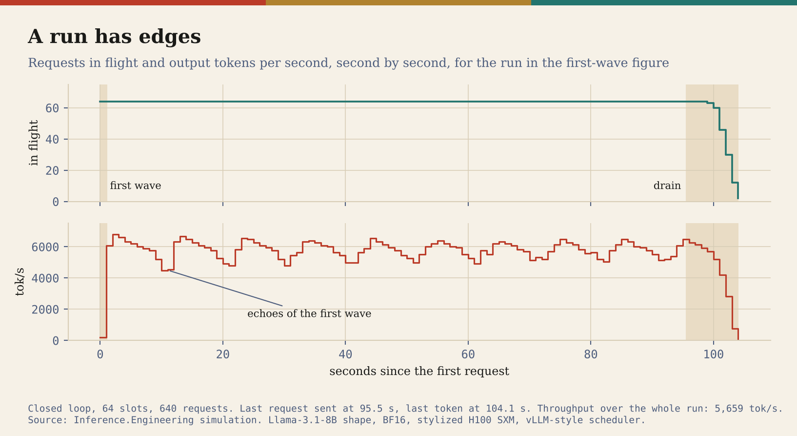
At ten times the concurrency, the throughput computed over the whole run is about 3% below the steady state. With a single wave, which is what you get when the number of prompts equals the concurrency, it is 9.5% below. The timeline also shows something I did not expect.
Because the members of the first wave finish at similar times, the slots they free get refilled at similar times, and the run keeps a dip every ten seconds or so, slowly damping, for the rest of its life.
SGLang’s benchmark now has a separate entry point that reports throughput over the longest interval where concurrency stays above a chosen fraction of its peak, which fixes this edge for throughput. GuideLLM goes even further: its warmup and cooldown are phases of the measured run itself, set as a duration, a request count or a fraction of the run, and every metric, latency percentiles included, is compiled only from the requests between them.
With a warmup long enough to cover the first wave, that removes the problem from the previous section as well.
The echo damps because the lengths vary. When they do not vary, it never damps.
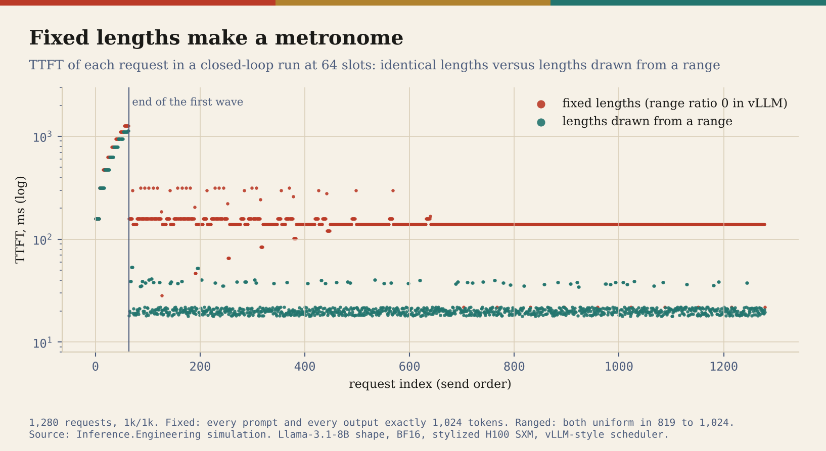
vLLM’s random dataset defaults to a range ratio of zero, which means every prompt has exactly the same length and, with --ignore-eos, so does every answer. In a closed loop that turns the benchmark into a metronome. Requests that start together finish together, so they get replaced together, and the run settles into cohorts.
In steady state, requests arrive in groups of 6.7 on average and up to 8, which is how many 1k prompts fit in one step’s budget. Every member of a cohort waits for the whole cohort’s prefill. With fixed lengths the steady-state median time to first token is 140 ms and the p99 is 316 ms.
Draw the lengths from a range and the same server, at the same concurrency, gives 20.1 ms and 40.2 ms.
There is one more trap in that flag. In upstream vLLM, a range ratio of r samples lengths uniformly between L(1 − r) and L(1 + r), and r has to be below 1. In the client InferenceX ships, which forked from an older version of vLLM’s script, the same flag samples between rL and L.
So the 0.8 in an InferenceX recipe means lengths between 80% and 100% of the nominal value, while the same 0.8 passed to upstream vllm bench serve means lengths between 20% and 180%. Reproducing a published point with the upstream tool and the published flags gives a different workload.
Open and closed
In 2006 Bianca Schroeder, Adam Wierman and Mor Harchol-Balter published a paper at NSDI called “Open Versus Closed: A Cautionary Tale”. In a closed system, a new request arrives only when a previous one completes, which is exactly what a fixed-concurrency benchmark does.
In an open system, requests arrive whether or not earlier ones have finished, which is what real users do. Their main finding was that at the same load the two give very different response times, that closed systems look much better, that the gap closes only slowly as concurrency grows, and that variability matters far more in open systems than in closed ones. They distilled eight principles from it.
To see how much of this carries over to an LLM server, I ran the same server both ways. The closed loop is a concurrency sweep from 1 to 256 slots, with twenty times the concurrency in prompts, measured in the steady window after the first wave.
The open loop is Poisson arrivals at a fixed rate, 4,000 to 8,000 requests per point, with the first and last 10% thrown away. Then, for each concurrency in the sweep, I ran the open loop at exactly the request rate the closed loop had delivered.
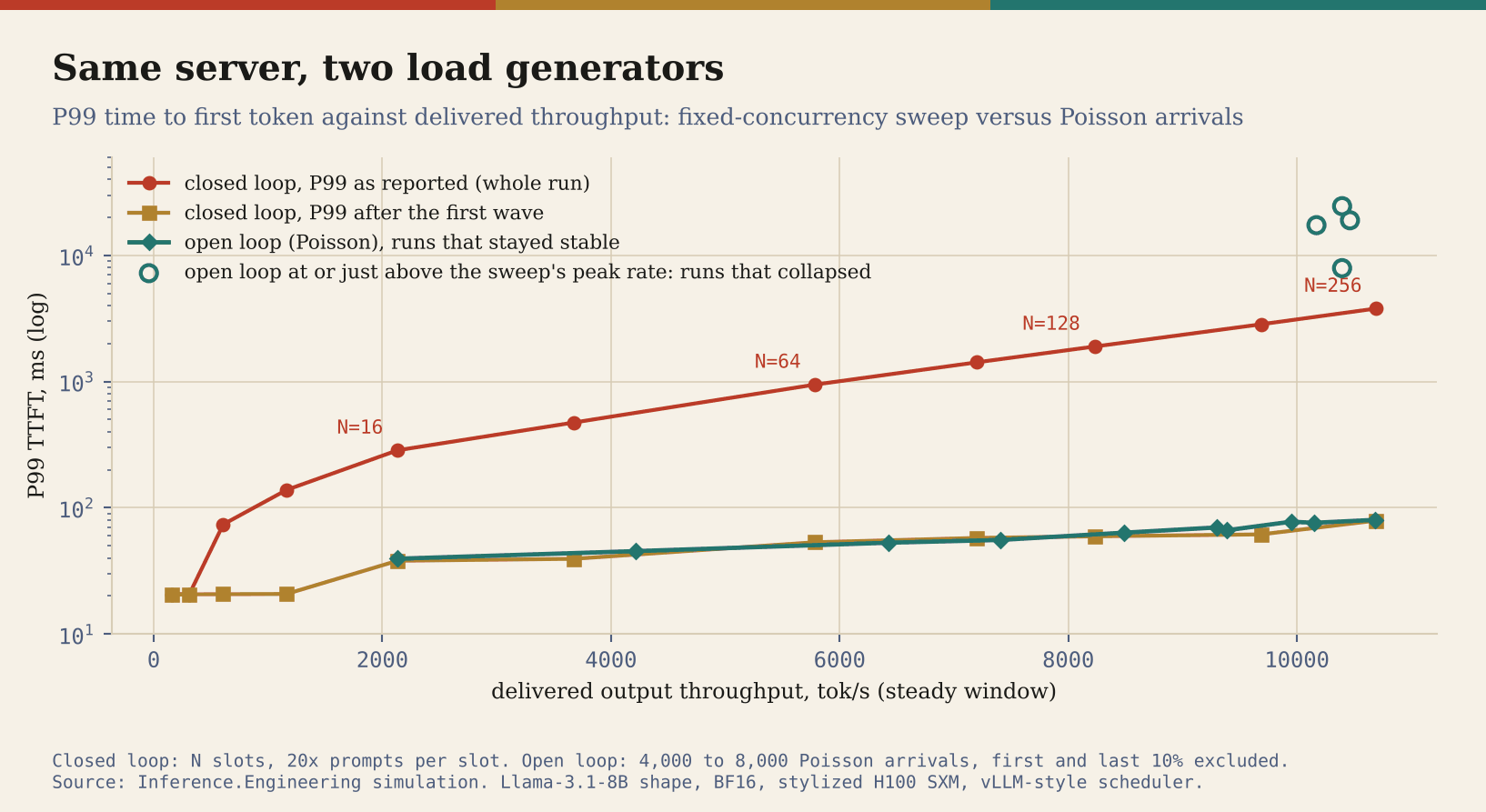
In the middle of the sweep, the two agree better than I expected. At 64 slots the closed loop delivers 6.29 requests per second with a steady-state p99 time to first token of 53.3 ms, and Poisson arrivals at the same rate give 51.5 ms. At 192 slots the open loop is 20% worse, 74.0 ms against 61.6 ms.
TPOT matches within a few percent, and the number of requests in the open system, averaged over time, is 65.5 when the closed loop held 64; Little’s law, the request rate times the mean latency, predicts 64.9 from the same run.
Continuous batching absorbs a burst by making the batch bigger rather than by making requests wait, so as long as there is room in the KV pool, arrivals that bunch up mostly cost everybody a little decode speed instead of costing somebody a long queue.
At small concurrency there is an artifact in the other direction. At 8 slots, Poisson arrivals give a p99 of 37.2 ms against 20.8 ms for the closed loop, 1.8 times worse.
A closed loop sends the next request exactly when the previous one finishes, which is always at the end of an engine step, so a new prompt never has to wait for the rest of a step that is already running. Real arrivals do not line up with the engine’s clock.
The interesting part is the top of the sweep. The closed loop peaks at 256 slots with 11.6 requests per second, 10,694 output tokens per second, and a steady-state p99 time to first token of 79 ms. That point is what a concurrency sweep reports as the capacity of the server.
I ran the open loop at that rate fifteen times with different seeds. Ten runs stayed fine, with p99s between 75 and 107 ms. The other five fell into the same failure.
The KV pool filled, the scheduler started preempting, every preempted request had to recompute its prompt and everything it had generated so far, which took capacity away exactly when there was none to spare, and the queue did not recover before the run ended. Their p99s were between 17.3 and 31.4 seconds, with between 1,429 and 2,825 preemptions each.
At 90%, 95% and 98% of the peak rate, all 14 runs at each load stayed clean, with p99s between 66 and 82 ms, and at 102% five of eleven spiraled.
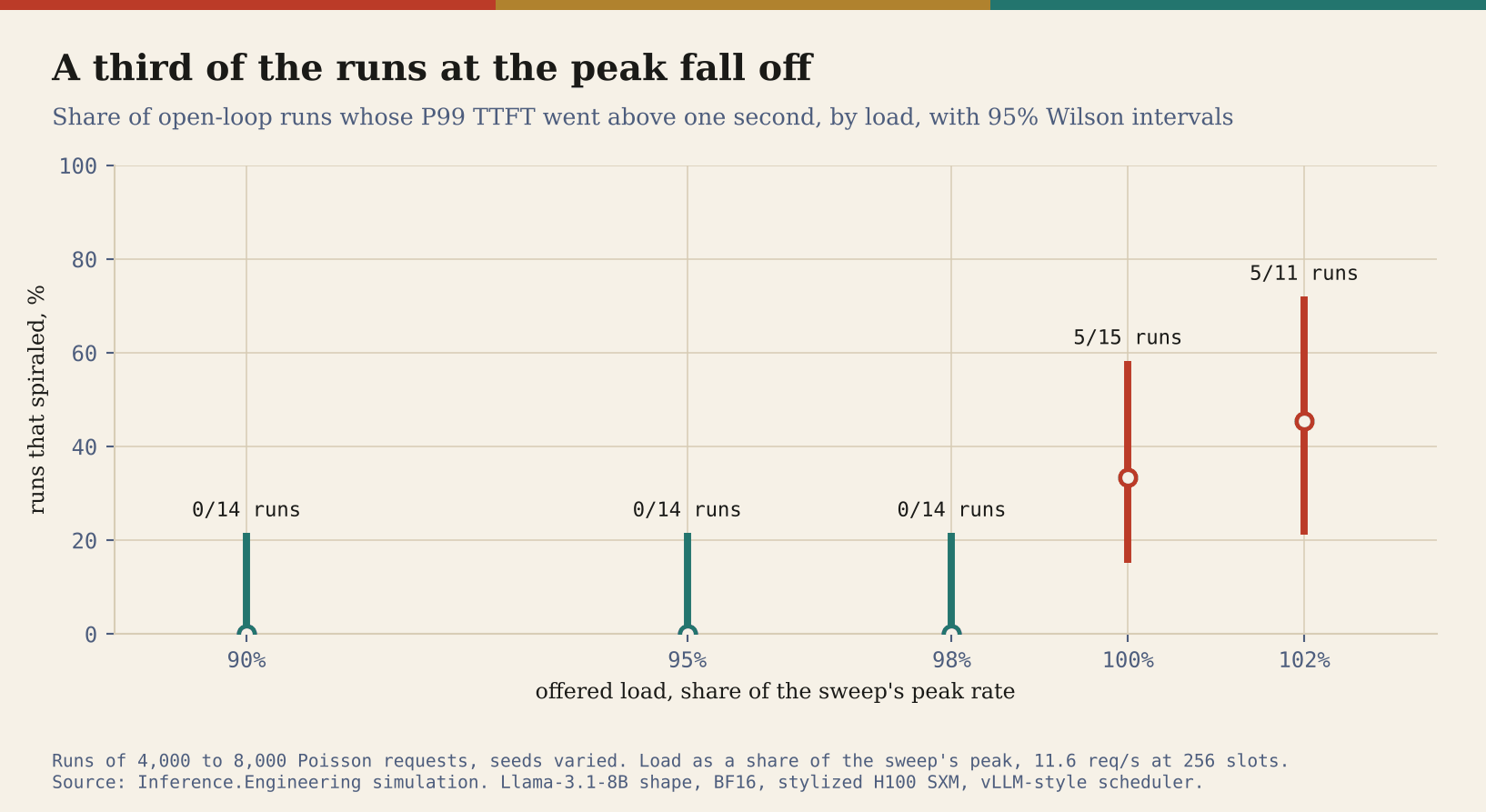
So the peak of the sweep is not a plateau. It is the edge of a cliff, and the closed loop cannot fall off it, because a closed loop never sends more work than the server just finished. Past the peak, the closed loop shows the cliff from the other side.
At 320 slots it delivers less, 10.98 requests per second, with 1,872 preemptions and a p99 of 10.9 s. But the point a sweep chart invites you to read as capacity is the highest one, and that is exactly the one that does not survive real traffic.
The peak of the sweep is not a plateau. It is the edge of a cliff, and the closed loop cannot fall off it.
The same paper offers a way to be fair to concurrency sweeps. Schroeder and her coauthors describe a partly-open model, where sessions arrive independently but the requests inside a session wait for each other, and they show it behaves like a closed system when sessions are long.
An agent making dozens of tool calls in a row is a long session. That makes the agentic track of InferenceX, which runs multi-turn agentic coding sessions built from traces over a fixed number of concurrent lanes, a more defensible use of a closed loop than a chat benchmark is.
Sessions still arrive independently of each other, though, so the cliff at the top applies to them as much as to chat requests.
The queue nobody times
vLLM’s client lets you combine a request rate with a concurrency cap. The help text explains that the cap simulates a higher level component enforcing a maximum, and that the actual rate may then be lower than requested if the server cannot keep up. What it does not say is when the clock starts.
In the code, the timer starts inside the request function, which runs after the semaphore is acquired. The time a request spends waiting for a slot is not part of its time to first token.
Gil Tene named this pattern coordinated omission more than a decade ago, in a talk called “How NOT to Measure Latency”. The load generator waits for the system, and so it never records the waiting it caused. A user who arrived on schedule and waited 30 seconds for a slot is recorded as a fast request.
A user who arrived on schedule and waited 30 seconds for a slot is recorded as a fast request.
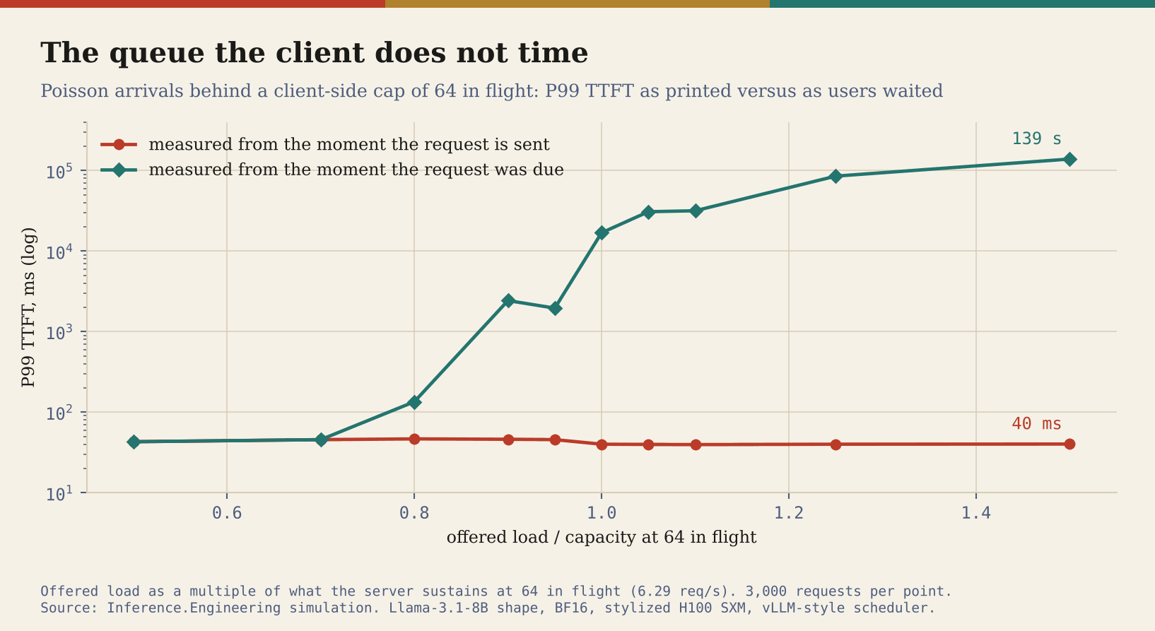
I put Poisson arrivals behind a client-side cap of 64 and swept the offered load around the throughput the server sustains at 64 in flight, which is 6.29 requests per second. Measured from the moment each request is sent, the p99 time to first token stays between 39 and 47 ms at every load, including one and a half times the capacity.
Measured from the moment each request was due, it is 135 ms at 80% load, 2.43 s at 90%, 16.9 s at 100% and 139 s at 150%, and in the overloaded cases it keeps growing with the length of the run. The achieved rate stops at 6.31 requests per second no matter what was offered.
The printed end-to-end p99 stays at 11.3 s while the experienced one reaches 149 s.
The tools are aware of this, and they are moving at different speeds.
The current vLLM client records the semaphore wait separately and, when both a rate and a cap are set, computes a queue-inclusive end-to-end latency, which it prints if you name it in
--percentile-metrics; its TTFT, its TPOT and its goodput still start the clock after the semaphore.SGLang’s benchmark took the same semaphore from vLLM, with a comment pointing at vLLM pull request 9390 from the autumn of 2024, and records nothing about the wait.
AIPerf reports an
effective_latencymeasured from the moment a request was issued, which its documentation calls “the only AIPerf latency metric that is coordinated-omission-aware”.GuideLLM reports a latency measured from the scheduled arrival, and refuses to compute it for closed-loop strategies, with a comment explaining that a delay measured against the system’s own responses would be “circular rather than a coordinated-omission correction”.
MLPerf’s LoadGen measures every Server-scenario latency from the scheduled time; in the current code, the latency of each sample is the delta from
scheduled_timeto completion.
Goodput deserves a sentence here because the word is doing double duty. In the DistServe paper, which vLLM’s own help text cites for the term, goodput is the highest request rate a system can serve while a target fraction of requests meet their TTFT and TPOT objectives.
In vLLM’s client, --goodput counts the requests that met the objectives and divides by the duration of the run, with latencies measured after the semaphore. Behind a client cap, the second one can report every request as good while users wait two minutes.
Percentiles
A p99 is an estimate, and it has a sample size. If requests were independent, there would be a clean, distribution-free answer to how much it can be trusted, because the number of samples below the true 99th percentile is binomial. The largest of n samples is a one-sided 95% upper bound on the true p99 only if n is at least 299.
With 100 requests, the largest one exceeds the true p99 only 63% of the time, so no order statistic of a 100-request run bounds the p99 at 95% confidence. For the p99.9 you need 2,995. With 1,000 requests, a two-sided 95% interval for the p99 runs from the 983rd to the 997th smallest value.
Two tools take this seriously. MLPerf’s LoadGen has an early-stopping rule built on the same binomial argument at 99% confidence, which lets a system that is clearly within its latency target finish with fewer queries and never lets one that misses it pass.
GuideLLM computes order-statistic intervals for its percentiles and refuses to print one when the sample cannot support it. Its docstring also says, plainly, that the interval describes how precisely the sample located the statistic and not how far it would move between runs.
That caveat is the one that matters, because requests in a serving benchmark are not independent. Requests that arrive close together share a queue, a batch and a prefill step. In an open-loop run at 90% of the sweep’s peak, the time to first token of one request has a correlation of 0.42 with the next one and 0.18 with the one after.
To measure what that does to a p99, I ran 160,000 requests at that load and cut the run into back-to-back windows the size of a typical benchmark, then compared the spread of the p99 across windows with the spread you would get by drawing the same number of requests independently from the whole run.
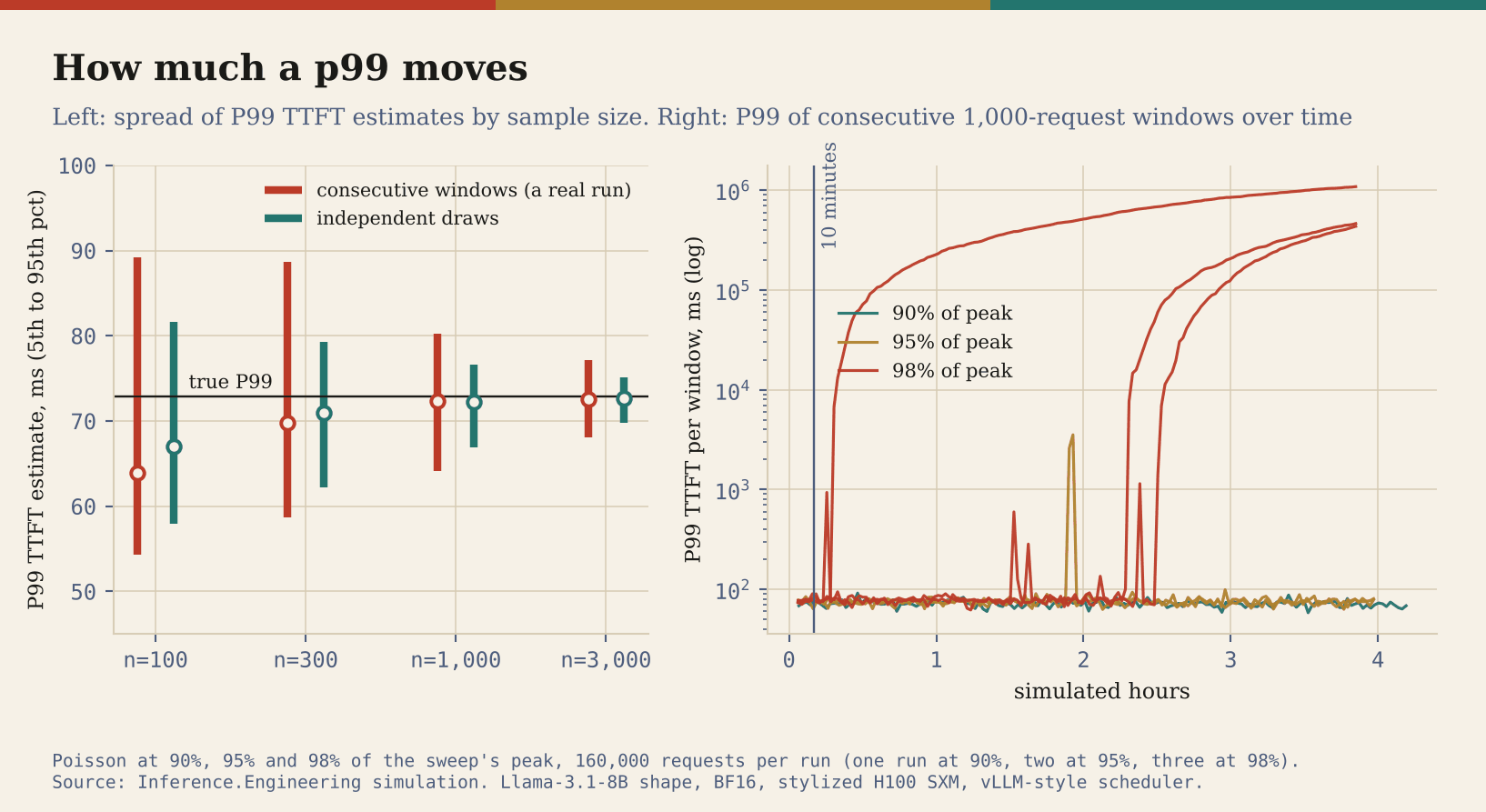
Consecutive windows of 1,000 requests have three times the variance of independent draws. The factor is 2.1 at 100 requests, 3.1 at 300, 3.0 at 1,000 and 3.5 at 3,000. In practice that means a 1,000-request run carries about as much information about its p99 as a third as many independent requests would.
The middle 90% of p99 estimates from consecutive 1,000-request windows runs from 64.1 to 80.3 ms, against 66.9 to 76.7 ms for independent draws, around a true value of 72.8 ms. At this load, any interval computed as if requests were independent is too narrow by a factor of about 1.7.
The right half of that figure is the result I did not expect. At 98% of the sweep’s peak, all 14 shorter runs from the previous section were clean. I then ran that rate three times for 160,000 requests each, about four simulated hours per run.
All three fell into the preemption spiral and none came back. One collapsed after 18 minutes, the others after 2.3 and 2.5 hours. The two later ones first went through transients, windows where the p99 jumped to between 0.3 and 1.1 seconds and came back down.
At 95%, one of two long runs had an episode just before the two-hour mark, with the windowed p99 reaching 3.5 seconds, and recovered; the other stayed clean, as did the single long run at 90%. In the first ten minutes of the three long runs at 98%, the worst 1,000-request window had a p99 of 90 ms.
A ten-minute benchmark, which is MLPerf’s minimum duration and 6,820 requests at that rate, would have seen a healthy server in all seventeen runs.
The failure has a name. Nathan Bronson and coauthors called it a metastable failure in a 2021 HotOS paper, describing a system that runs fine at a given load, gets knocked into a bad state by a transient, and stays there because the bad state sustains itself.
Recompute preemption is a clean example of the mechanism, since it spends capacity precisely when capacity is short. A real deployment would add its own feedback on top, timeouts and retries that make it worse or admission control and load shedding that make it better, but the shape is the same.
What decides whether a rate is safe is how the system recovers from its worst minute, and only a long run is likely to contain one.
What decides whether a rate is safe is how the system recovers from its worst minute, and only a long run is likely to contain one.
There is a cost version of this. A cost per million tokens is a price per GPU-hour divided by the tokens a GPU produces in that hour, so it inherits whatever throughput sits in the denominator.
At 90% of the sweep’s peak, where a four-hour run stayed healthy from start to finish, every token costs 11% more, at the same price per GPU-hour, than the peak suggests. The real price of serving this workload is somewhere between those two numbers, and a short benchmark cannot say where.
How much of this is the model
Every effect so far comes from one set of constants, and constants are where a simulator hides its opinions. So I measured four of the effects again under eleven versions of the model, changing one thing at a time: compute efficiency at 60, 75 and 90%, bandwidth efficiency at 75, 85 and 95%, step overhead at half a millisecond, one and two, the KV pool at 300,000, 430,000 and 600,000 tokens, and the token budget at 2,048, 8,192 and 16,384.
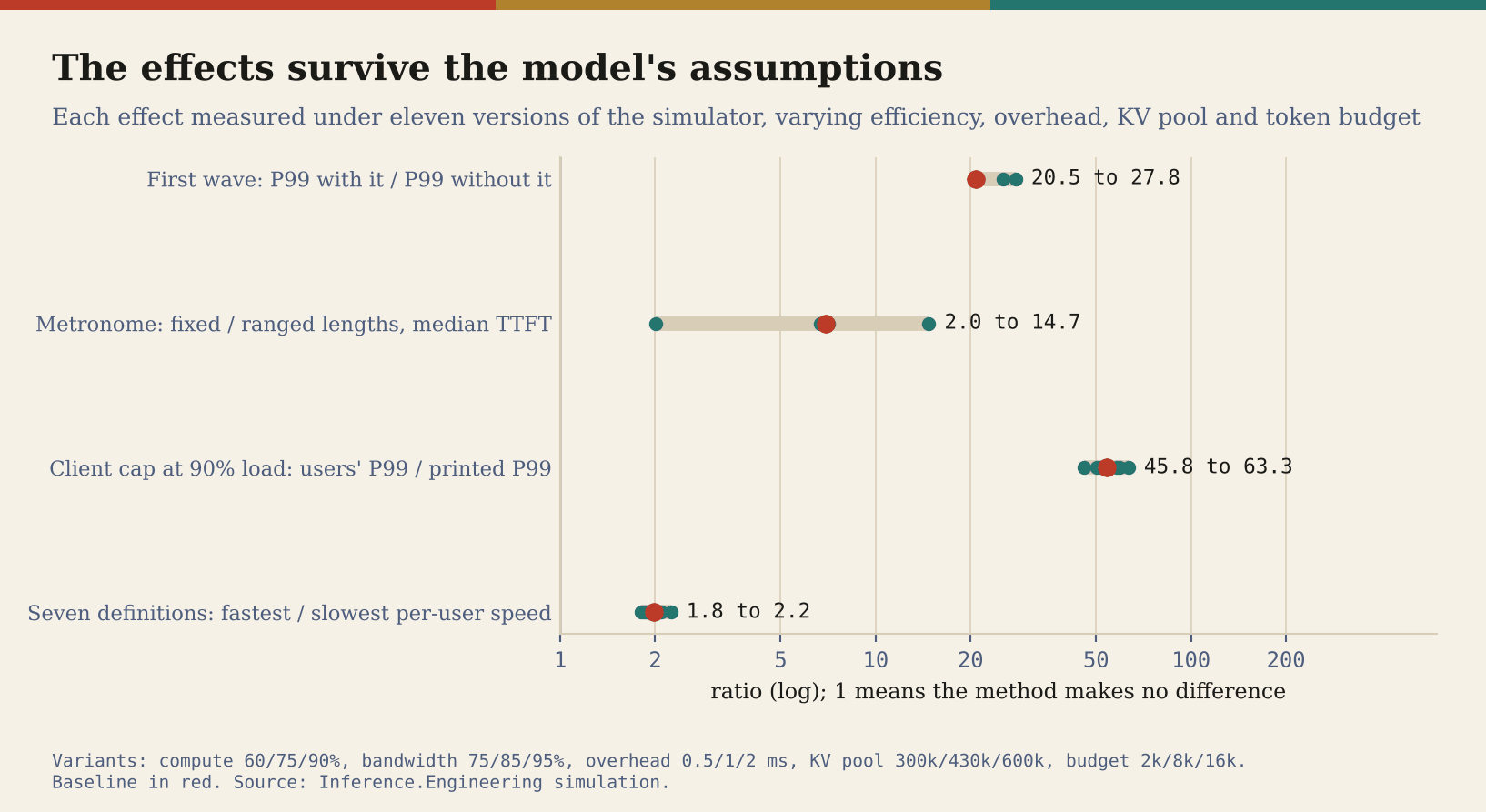
None of the effects goes away.
The first wave inflates the p99 between 20.5 and 27.8 times.
Behind a client cap at 90% load, users wait between 46 and 63 times longer at the p99 than the printed number says, and between half load and 125% load the printed p99 does not rise; it falls by 5 to 12%.
The seven definitions disagree by a factor between 1.8 and 2.2.
The metronome is the one effect that depends strongly on a setting, because a cohort can be as large as the number of prompts that fit in one step. With fixed lengths, the median time to first token is 2.0 times the ranged one under a 2,048-token budget and 14.7 times under 16,384.
The KV pool changes none of these numbers, because none of these experiments runs out of KV cache. It does decide where the cliff is, and I did not sweep that.
What a token is
Tokens per second is the unit everything is quoted in, and a token is not a unit. To put numbers on that I measured seven real tokenizers offline, using llama.cpp’s llama-tokenize against the vocab-only GGUF files that llama.cpp keeps for its own tokenizer tests, on three kinds of text: 1.44 million characters of English technical documentation, the same text of about 540 words written in English and in Italian, and the CPython 3.11 asyncio package.
Tokens per second is the unit everything is quoted in, and a token is not a unit.
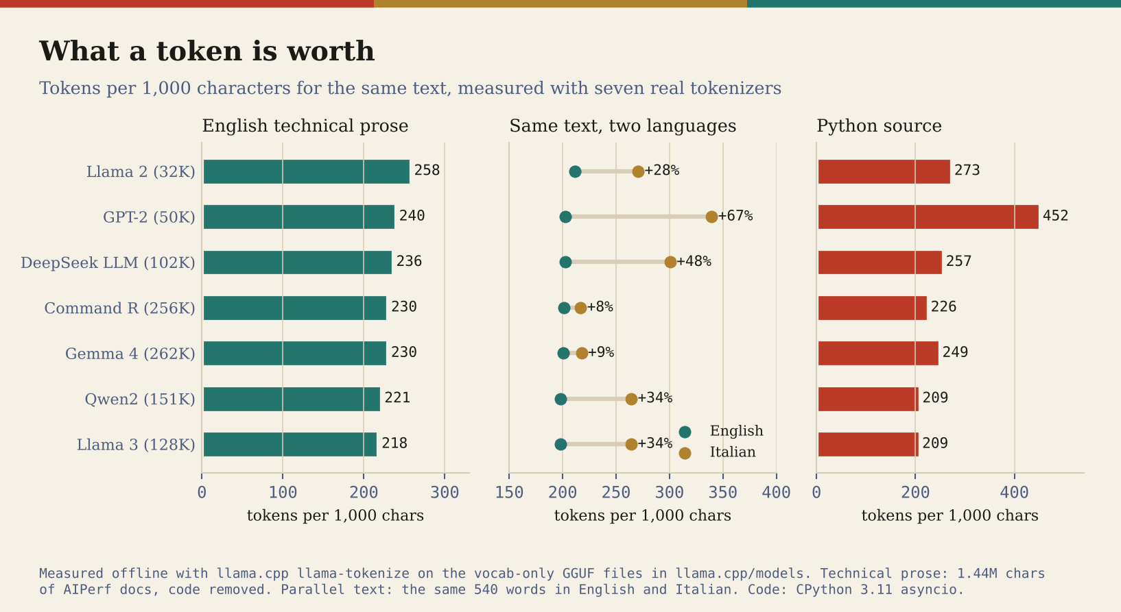
On English technical prose, Llama 3’s tokenizer needs 217.9 tokens per 1,000 characters and Llama 2’s needs 258.0, so Llama 3 writes the same text in 15.6% fewer tokens. Meta’s own launch post said up to 15%, and on this corpus that is about what it is. On Python the gap is wider.
Llama 2 needs 1.31 times the tokens, and GPT-2’s tokenizer, which was not built with code in mind and handles indentation poorly, needs 2.17 times. Language can matter as much as the tokenizer.
The same paragraph in Italian costs 34% more tokens than in English under Llama 3, 67% more under GPT-2, and only about 9% more under Gemma 4’s 262,000-entry vocabulary. The same Italian paragraph costs 21% more tokens under Llama 3 than under Gemma 4.
This is why LLMPerf’s choice matters. Its README says tokens are counted with the Llama tokenizer whatever API is being tested, so that prompts stay consistent, and the code loads the 32,000-entry tokenizer that Llama 1 and Llama 2 share, for prompts and outputs alike. That is a sensible choice when comparing providers who serve the same model.
Across models it is a foreign unit. For a Llama 3 model writing English technical text, LLMPerf reports 18.4% more tokens than the model generated, and on code 31% more, so its tokens per second are inflated by the same factor.
The only fair cross-model comparison I know of is characters or bytes of output per second, measured on the same kind of text, with the language stated.
Reasoning models add a second ambiguity. A model that thinks for 900 tokens before answering in 100 has a time to first token measured on its first thinking token, and a tokens-per-second figure that counts tokens the user may never see.
AIPerf reports a separate time to first output token, from the start of the request to the first non-reasoning token. When the answer is what the user waits for, that is the number to print.
What the prompt is
vLLM’s random dataset does not contain random text. Its docstring says the prompt tokens are generated as (offset + index + arange(input_len)) % vocab_size, then decoded and re-encoded to fix the length. That is a random starting point followed by consecutive token IDs, a staircase walking through the vocabulary.
The client InferenceX ships builds its prompts with the same formula. Neither looks like anything a user would type, and for some measurements that matters a great deal.
InferenceX’s maintainers say so in their own repository. The README for their speculative decoding policy explains that random-token inputs can distort acceptance behavior, expert routing, and measured throughput, and describes what they did about it.
For each model and draft length they measure a mean acceptance length on the coding category of SPEED-Bench, a speculative decoding benchmark built from real prompts, and then force every engine to accept drafts at exactly that average length.
vLLM has a synthetic rejection sampler with a synthetic_acceptance_length option for this; I checked that it exists in vLLM’s speculative config.
SGLang has an environment variable that simulates an acceptance length, and TensorRT-LLM has one that forces the number of accepted draft tokens, which according to the README excludes the bonus token, so it has to be set to the golden acceptance length minus one.
I think this is the right decision, and it is worth noticing what it means. A benchmark that much of the industry quotes now simulates part of the model’s behavior inside the engine, by policy, because acceptance measured on synthetic prompts would describe text no user ever sends.
A speculative decoding result from it is a statement of the form “this fast, given an acceptance length of x”, and the x deserves to be printed next to the speed.
The SPEED-Bench authors report that synthetic inputs overestimate real-world throughput and that the best draft length depends on batch size, which is one more reason to want the clause.
Mixture-of-experts models have their own version of the problem. If routing were uniform, a batch of 32 tokens in a DeepSeek-V3-style layer, with 256 routed experts and 8 chosen per token, would touch 63.8% of the experts; a batch of 128 would touch 98.3%. Past a hundred or so tokens per step, a decode step reads nearly all of the expert weights, so the active parameter count is a batch-one number, not a description of what a serving step costs.
Real routing is not uniform, and how skewed it is decides how many experts each step reads and how evenly the load spreads across GPUs in expert parallelism. A staircase of token IDs is not a neutral input to that.
The last thing synthetic prompts change is the cache. Random prompts share no prefix, so a prefix cache never hits. Agents are the opposite.
Manus wrote in 2025 that its average ratio of input to output tokens is around 100 to 1 and called the KV-cache hit rate “the single most important metric for a production-stage AI agent”, which makes sense when cached input costs a tenth of uncached input on the API they used.
A benchmark built on random prompts measures a workload where nothing is reused, which is the opposite of how agents use a server.
Two checks anyone can run
Most of what I have described requires reading code or running experiments. Two checks require neither, and they are worth running on any table before trusting it.
The first is Little’s law: the average number of requests in a system equals the arrival rate times the average time each one spends inside. A closed loop with no think time keeps exactly N requests in flight, so its throughput in requests per second times its mean end-to-end latency has to come out at N.
In the simulator, at 64 slots, 6.287 requests per second times 10.172 seconds is 64.0. If a table claims 64 concurrent users, 6 requests per second and a mean latency of 30 seconds, one of the three numbers is wrong or was measured over a different window.
SGLang’s benchmark prints concurrency computed exactly this way, as the sum of latencies over the duration, which makes the check free.
The second is the roofline. A decode step has to read every weight and every token of KV cache it attends to, so a single user can never be served faster than memory bandwidth divided by the bytes read per step. For an 8B model in BF16 on an H100 that is 3.35 TB/s over 15.0 GB, 223 tokens per second at batch one, before any overhead.
Add users and the per-user speed falls while the total rises, until the weight matrices become compute-bound, which for BF16 on an H100 happens at around 295 tokens per step.
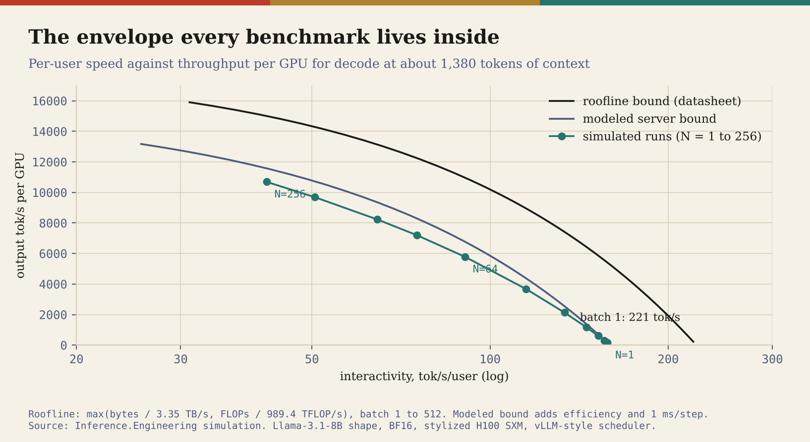
Every BF16 run of this model on this GPU without speculation lands inside that envelope. The simulated runs sit below the modeled bound because some of their steps are spent on prefill.
A published point outside the envelope is not necessarily wrong, but it is reading fewer bytes per token than the envelope assumes, through quantization, speculation or sparsity, and the result should say which.
Flags that already exist
Most of these problems already have a remedy inside the tools, usually behind a flag that is not the default. This is what I would set today, at the commits I read.
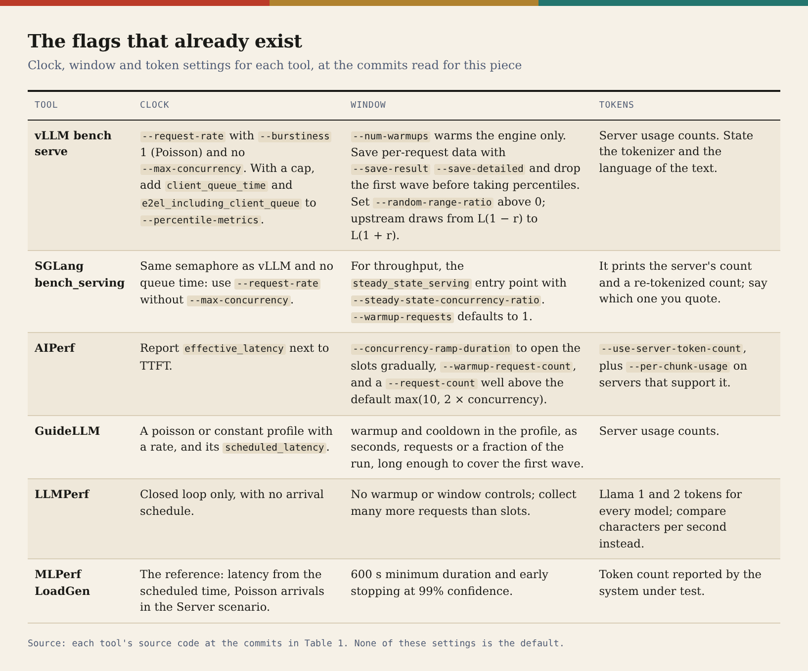
None of this needs new software, only the flags and a line in the write-up saying they were used.
What I write next to a number now
After all of this, I do not think the answer is to stop publishing benchmark numbers. The answer is to publish the clauses that decide what they mean. These are the ones I now write next to every number I quote, my own or anyone else’s:
Arrivals: a rate and its distribution, or a concurrency and how the run starts. A fixed concurrency with every slot opening at once should say so.
Clock: whether latency starts when a request was due, when it was sent, or when the server accepted it.
Window: which parts of the run were excluded, such as warmup, the first wave and the drain, and how long the run was, in requests and in time.
Definitions: the formula behind each per-token metric, because the names do not carry it, and the sample size and interval behind each percentile.
Tokens: whose tokenizer, whether reasoning tokens are included, and the language of the text.
Prompts: where they came from, how their lengths were drawn, and the prefix cache hit rate.
Speculation: measured acceptance on named data, or an injected acceptance length.
Quality: accuracy at the same configuration, since quantization, speculation and batch-dependent numerics all change outputs. Thinking Machines showed in 2025 that 1,000 completions of the same prompt at temperature zero on Qwen3-235B, served by vLLM, produced 80 distinct answers, because the batch a request lands in changes its arithmetic.
Versions: the commit of the tool and of the engine. Five of the seven tools in this piece had commits in the three days before I read them.
It is a long list, but most of it fits in two lines under a chart, and without it I no longer know what a number means.
Where I might be wrong
The simulator is a model, and some of its effects are sharper than reality would allow.
Network jitter, HTTP parsing and SSE framing would loosen the cohorts in the metronome experiment and blur the steps of the first wave, though not the arithmetic of the wave itself, which only depends on how much prompt has to be prefilled before the last request gets its turn.
Real engines also have asynchronous scheduling, CPU overhead that varies with batch composition, and kernels whose efficiency depends on shape in ways a roofline does not capture.
The efficiency constants are mine, not measurements, so absolute capacities and the location of the cliff could sit elsewhere on real hardware. The ratios in the section on the model’s assumptions are the numbers I would defend, more than any absolute value.
The scheduler is vLLM-like, not vLLM. I did not model prefix caching in these runs, request priorities, KV offloading or the details of how vLLM batches prefill chunks. SGLang reserves memory and schedules differently, and TensorRT-LLM differently again.
The sensitivity sweep changes one constant at a time and never touches the scheduling policy. The cliff at the top of the sweep depends on recompute preemption with no admission control; a system that swaps KV to host memory, or sheds load, would fail differently, possibly more gracefully.
I modeled InferenceX’s client parameters on one simulated GPU. I did not run anything on their hardware, so I do not know how much of any published p99 time to first token is first wave. The formula in that section, concurrency times mean prompt length over prefill throughput, lets anyone check a published point against it.
On large multi-GPU systems the prefill rate is much higher and the effect smaller in milliseconds, though not in kind. The same goes for AIPerf’s default and the NIM quickstart. I replayed their request counts on the simulator, not anybody’s published runs.
I read every tool at a specific commit, listed in the table and the dossier. These are fast-moving projects, and some of what I describe, like vLLM’s queue-inclusive latency, appeared recently enough that it may change again soon. If I misread any tool’s behavior, I would like to know, and I will correct it here.
The tokenizer measurements are exact for the files I used, but the parallel English and Italian text is short, about 540 words that I wrote myself, and the English technical corpus is documentation, not chat. Ratios on other text will differ by a few percent.
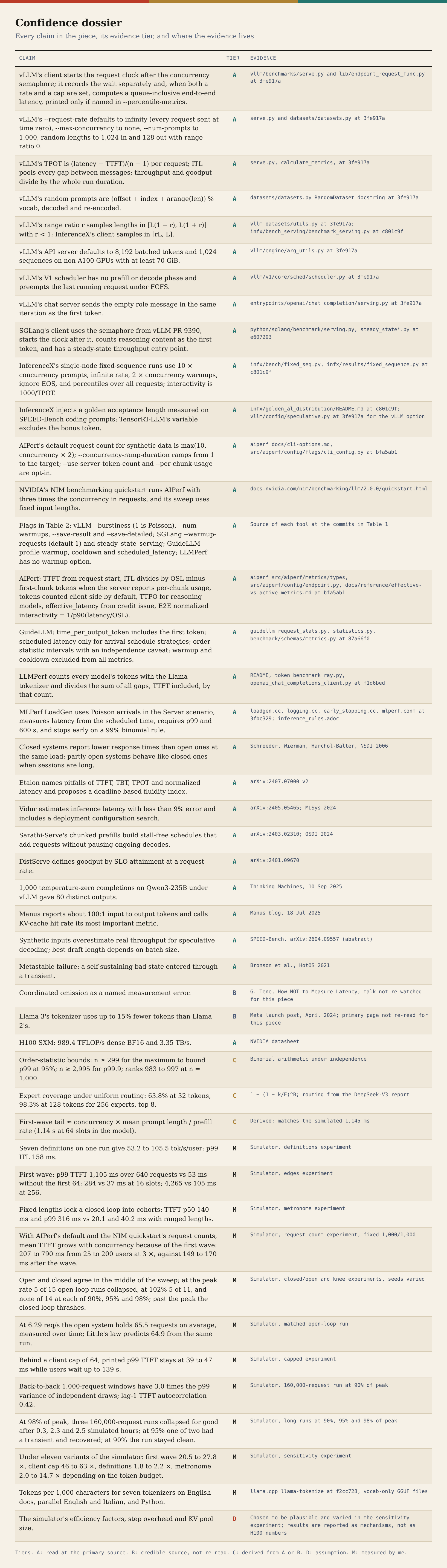
Confidence dossier
Sources
vLLM project. vllm bench serve: vllm/benchmarks/serve.py, lib/endpoint_request_func.py, datasets/. Commit 3fe917a, 11 October 2026. github.com/vllm-project/vllm
vLLM project. vllm/engine/arg_utils.py, vllm/v1/core/sched/scheduler.py, vllm/entrypoints/openai/chat_completion/serving.py, vllm/config/speculative.py. Commit 3fe917a.
R. Bryant. “[Misc] benchmark: Add option to set max concurrency”. vLLM pull request 9390, 2024. github.com/vllm-project/vllm/pull/9390
SGLang project. python/sglang/benchmark/serving.py and steady_state_serving.py. Commit e607293, 11 October 2026. github.com/sgl-project/sglang
SemiAnalysis. InferenceX: inferencex-e2e/infx/bench/fixed_seq.py, infx/bench_serving/, infx/results/fixed_sequence.py, infx/golden_al_distribution/README.md, docs/agentx-standalone.md. Commit c801c9f, 10 October 2026. github.com/SemiAnalysisAI/InferenceX
SemiAnalysis. InferenceX, formerly InferenceMAX: about page. inferencex.semianalysis.com/about
NVIDIA. AIPerf: src/aiperf/metrics/types/, src/aiperf/config/flags/cli_config.py, docs/cli-options.md and docs/reference/effective-vs-active-metrics.md. Commit bfa5ab1, 11 October 2026. github.com/ai-dynamo/aiperf
NVIDIA. NIM LLM benchmarking guide: AIPerf quickstart. docs.nvidia.com/nim/benchmarking/llm/2.0.0/quickstart.html
GuideLLM: src/guidellm/schemas/base/request_stats.py and statistics.py, src/guidellm/benchmark/schemas/metrics.py, src/guidellm/schemas/benchmark/transient.py and profiles/. Commit 87a66f0, 9 October 2026. github.com/vllm-project/guidellm
Ray project. LLMPerf: README, token_benchmark_ray.py, src/llmperf/ray_clients/openai_chat_completions_client.py. Commit f1d6bed, 8 December 2024. github.com/ray-project/llmperf
MLCommons. MLPerf Inference LoadGen v6.0.17: loadgen.cc, logging.cc, early_stopping.cc, mlperf.conf. Commit 3fbc329, 2 September 2026. github.com/mlcommons/inference
MLCommons. MLPerf Inference rules, including the early stopping criterion. github.com/mlcommons/inference_policies
V. J. Reddi et al. “MLPerf Inference Benchmark”. ISCA 2020. arXiv:1911.02549
B. Schroeder, A. Wierman, M. Harchol-Balter. “Open Versus Closed: A Cautionary Tale”. NSDI 2006. usenix.org
G. Tene. “How NOT to Measure Latency”. QCon San Francisco 2012, and later versions of the talk.
A. Agrawal, A. Agarwal, N. Kedia, J. Mohan, S. Kundu, N. Kwatra, R. Ramjee, A. Tumanov. “Etalon: Holistic Performance Evaluation Framework for LLM Inference Systems”. 2024. arXiv:2407.07000
A. Agrawal, N. Kedia, J. Mohan, A. Panwar, N. Kwatra, B. Gulavani, R. Ramjee, A. Tumanov. “Vidur: A Large-Scale Simulation Framework for LLM Inference”. MLSys 2024. arXiv:2405.05465
A. Agrawal, N. Kedia, A. Panwar, J. Mohan, N. Kwatra, B. S. Gulavani, A. Tumanov, R. Ramjee. “Taming Throughput-Latency Tradeoff in LLM Inference with Sarathi-Serve”. OSDI 2024. arXiv:2403.02310
Y. Zhong et al. “DistServe: Disaggregating Prefill and Decoding for Goodput-optimized Large Language Model Serving”. OSDI 2024. arXiv:2401.09670
N. Bronson, A. Aghayev, A. Charapko, T. Zhu. “Metastable Failures in Distributed Systems”. HotOS 2021.
T. Abramovich et al. “SPEED-Bench: A Unified and Diverse Benchmark for Speculative Decoding”. 2026. arXiv:2604.09557
H. He and Thinking Machines Lab. “Defeating Nondeterminism in LLM Inference”. 10 September 2025. thinkingmachines.ai
Y. Ji. “Context Engineering for AI Agents: Lessons from Building Manus”. 18 July 2025. manus.im
Meta. “Introducing Meta Llama 3”. April 2024. ai.meta.com
llama.cpp: tools/tokenize and models/ggml-vocab-*.gguf. Commit f2cc728, 11 October 2026. github.com/ggml-org/llama.cpp
DeepSeek-AI. “DeepSeek-V3 Technical Report”. arXiv:2412.19437
J. D. C. Little. “A Proof for the Queuing Formula: L = λW”. Operations Research 9(3), 1961.
NVIDIA. H100 Tensor Core GPU datasheet.
Appendix: the model
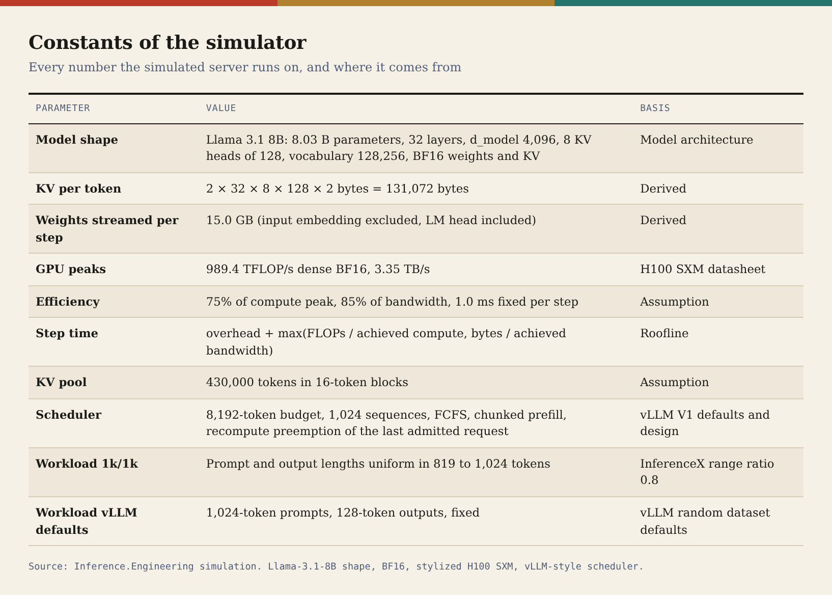
Every simulated number in this piece comes from the two functions below, driven with fixed seeds. The rest of the code builds workloads, applies each tool’s metric definitions to the recorded timestamps, and draws the figures; each figure’s footer states its experiment.
def step_time(cfg: ServerConfig, n_tok: int, n_logits: int, attn_ctx_sum: float,
              prefill_attn_pairs: float, kv_read_tokens: float) -> float:
    m, hw = cfg.model, cfg.hw
    flops = 2.0 * m.body_params * n_tok + 2.0 * m.lm_head_params * n_logits
    flops += 4.0 * m.layers * m.d_model * (attn_ctx_sum + prefill_attn_pairs)
    bytes_ = m.streamed_weight_bytes + m.kv_bytes_per_token * (kv_read_tokens + n_tok)
    t_c = flops / (hw.eta_compute.value * hw.peak_flops.value)
    t_m = bytes_ / (hw.eta_memory.value * hw.hbm_bw.value)
    return hw.step_overhead_s.value + max(t_c, t_m)


def run(cfg: ServerConfig, isl, osl, client: dict, cached=None,
        record_tokens: bool = True, record_steps: bool = False):
    """Simulate one benchmark.

    client kinds:
      open    {"kind": "open", "times": [...]}            arrivals independent of the server
      closed  {"kind": "closed", "N": n}                  n slots, next request on completion,
                                                            every request logically arrives at t=0
      capped  {"kind": "capped", "times": [...], "cap": c} scheduled arrivals behind a FIFO
                                                            semaphore of size c (client side)
    """
    n = len(isl)
    reqs = [Req(i, int(isl[i]), int(osl[i]), int(cached[i]) if cached is not None else 0)
            for i in range(n)]
    kind = client["kind"]
    if kind in ("open", "capped"):
        times = np.asarray(client["times"], dtype=float)
        for r, ts in zip(reqs, times):
            r.sched_t = float(ts)
    else:
        for r in reqs:
            r.sched_t = 0.0

    bs = cfg.block_size
    free_blocks = cfg.kv_capacity_tokens // bs
    waiting: deque = deque()
    running: list = []
    t = 0.0
    nxt = 0            # next request index the client has not dispatched or queued
    inflight = 0       # client view: sent and not finished
    client_q: deque = deque()
    done = 0
    steps = [] if record_steps else None
    preemptions = 0
    cap = client.get("cap")
    N = client.get("N")

    def send(r, ts):
        nonlocal inflight
        r.send_t = ts
        inflight += 1
        waiting.append(r)

    # initial dispatch
    if kind == "closed":
        while nxt < n and inflight < N:
            send(reqs[nxt], 0.0)
            nxt += 1

    def dispatch_arrivals(upto):
        """Open and capped clients: handle scheduled arrivals with time <= upto, in order."""
        nonlocal nxt
        while nxt < n and reqs[nxt].sched_t <= upto:
            r = reqs[nxt]
            nxt += 1
            if kind == "open":
                send(r, r.sched_t)
            else:
                if inflight < cap and not client_q:
                    send(r, r.sched_t)
                else:
                    client_q.append(r)

    while done < n:
        if kind in ("open", "capped"):
            dispatch_arrivals(t)
        if not running and not waiting:
            # idle server: jump to the next arrival
            if kind in ("open", "capped") and nxt < n:
                t = max(t, reqs[nxt].sched_t)
                continue
            raise RuntimeError("deadlock: nothing running, nothing to send")

        # ---------------- schedule one step ----------------
        budget = cfg.token_budget
        sched = []          # (req, n_new)
        preempted_now = False
        i = 0
        while i < len(running) and budget > 0:
            r = running[i]
            need = r.isl + r.gen - r.computed
            n_new = need if need <= budget else budget
            want_blocks = -(-(r.computed - r.cached + n_new) // bs) - r.blocks
            while want_blocks > free_blocks:
                victim = running.pop()
                free_blocks += victim.blocks
                victim.blocks = 0
                victim.computed = victim.cached
                victim.npre += 1
                preemptions += 1
                preempted_now = True
                waiting.appendleft(victim)
                if victim is r:
                    break
            else:
                free_blocks -= want_blocks
                r.blocks += want_blocks
                sched.append((r, n_new))
                budget -= n_new
                i += 1
                continue
            # r itself was preempted; running shrank past i
            break

        if not preempted_now:
            while waiting and budget > 0 and len(running) < cfg.max_num_seqs:
                r = waiting[0]
                need = r.isl + r.gen - r.computed
                n_new = need if need <= budget else budget
                want_blocks = -(-(r.computed - r.cached + n_new) // bs) - r.blocks
                if want_blocks > free_blocks:
                    break
                waiting.popleft()
                free_blocks -= want_blocks
                r.blocks += want_blocks
                running.append(r)
                sched.append((r, n_new))
                budget -= n_new

        if not sched:
            # nothing fits (should not happen with a sane KV pool)
            raise RuntimeError("no request could be scheduled")

        # ---------------- cost of the step ----------------
        n_tok = 0
        n_logits = 0
        attn_ctx = 0.0
        pre_pairs = 0.0
        kv_read = 0.0
        n_dec = 0
        for r, k in sched:
            n_tok += k
            c0 = r.computed
            if r.computed + k == r.isl + r.gen:
                n_logits += 1
            if k == 1 and c0 > 0:
                attn_ctx += c0 + 1
                kv_read += c0
                n_dec += 1
            else:
                pre_pairs += k * c0 + k * (k + 1) / 2.0
                kv_read += c0
        dt = step_time(cfg, n_tok, n_logits, attn_ctx, pre_pairs, kv_read)
        t_end = t + dt
        if steps is not None:
            steps.append((t, dt, n_dec, n_tok - n_dec, len(running), len(waiting),
                          cfg.kv_capacity_tokens // bs - free_blocks))

        # arrivals during the step are dispatched before completions at t_end
        if kind in ("open", "capped"):
            dispatch_arrivals(t_end)

        # ---------------- apply the step ----------------
        finished = []
        for r, k in sched:
            r.computed += k
            if r.computed == r.isl + r.gen:
                r.gen += 1
                if r.first_t is None:
                    r.first_t = t_end
                if record_tokens:
                    r.tok_times.append(t_end)
                if r.gen >= r.osl:
                    r.finish_t = t_end
                    finished.append(r)
        if finished:
            fin = set(id(r) for r in finished)
            running = [r for r in running if id(r) not in fin]
            for r in finished:
                free_blocks += r.blocks
                r.blocks = 0
                done += 1
                inflight -= 1
            if kind == "closed":
                while nxt < n and inflight < N:
                    send(reqs[nxt], t_end)
                    nxt += 1
            elif kind == "capped":
                while client_q and inflight < cap:
                    send(client_q.popleft(), t_end)
        t = t_end

    out = {
        "reqs": reqs,
        "preemptions": preemptions,
        "steps": steps,
    }
    return out