



The short version
On day zero the config is the only spec sheet you have. Seven numbers that come straight from it decide how a model serves: resident parameters, active parameters, bytes per step, KV bytes per token, expert coverage, the attention crossover and node capacity.
Muse Spark Open’s launch shows what goes wrong without them. Its launch post sized a million token cache with all 62 layers and got 266 GB. Only 16 layers are global, so the real figure is 69.1 GB in BF16 and 34.6 GB in FP8.
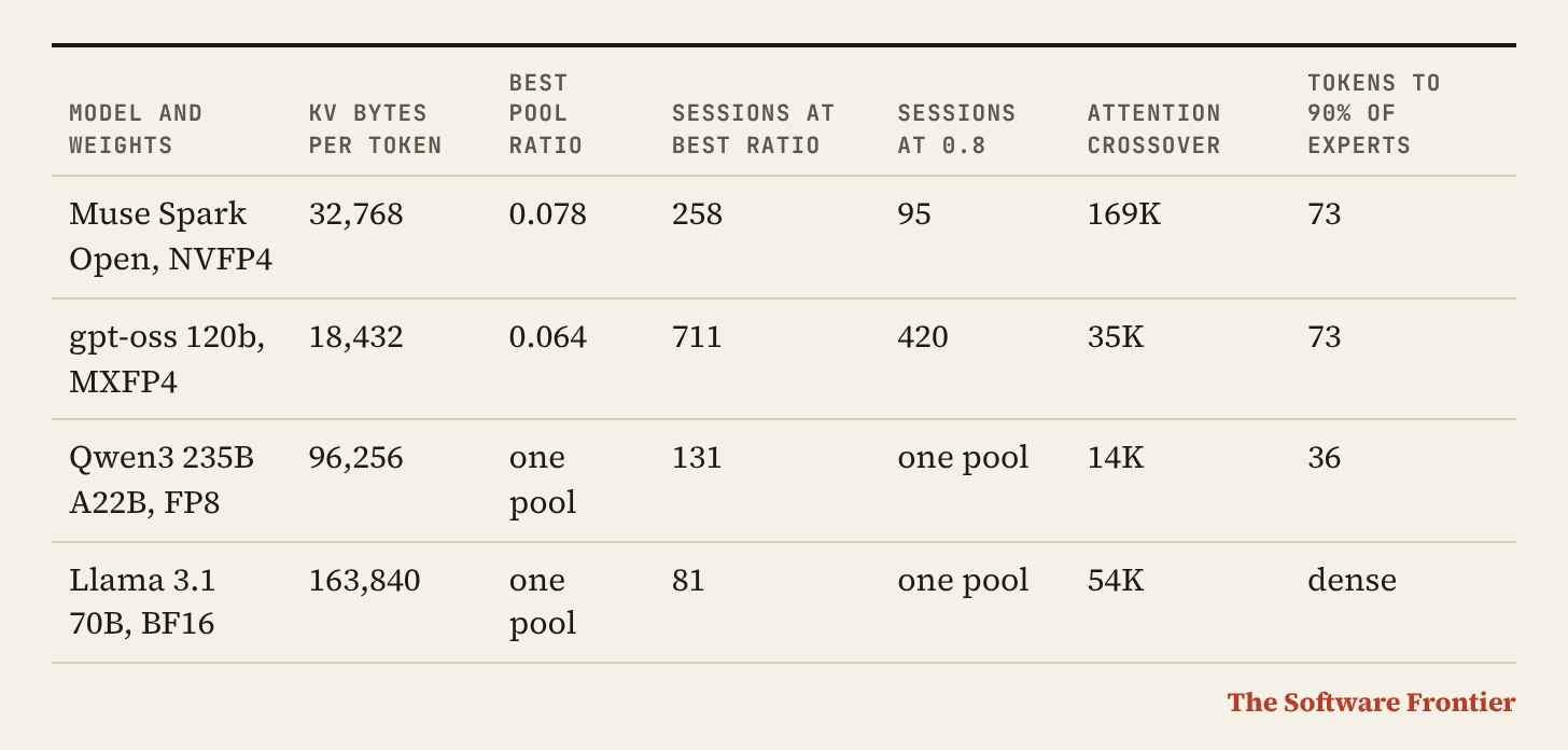
Hybrid attention needs a memory decision that dense models never asked for. SGLang splits the KV cache into a full pool and a sliding pool with one ratio. For long sessions on Muse Spark Open the default gives 70% of the memory to layers that hold 2,048 tokens, and a node fits 95 sessions at 128K instead of 258. The right ratio is the window plus one prefill chunk, divided by the mean context of the sessions the node holds.
Speculative decoding costs more bytes on a fine grained MoE. An 8 token verify block reads 7.2 times the expert weights of a plain step at one request and 1.6 times at 32. Measured gains on MI355X fell from about 70% at low concurrency to 6% and 31% at 32 requests, for the two launch drafters.
Benchmarks report what is easy to count. The headline 80.3K tokens per second per GPU is 0.27% output, and at 128 sessions an agent waits 12.4 of its 16 seconds per turn before the first token.
The cache is a pricing decision. Holding a session’s cache pays for itself if the agent returns within 4.9 to 6.9 minutes on rented B300s at list prices, almost independent of context length.
We are releasing LLM Systems Engineering, the guide where we work through this method and the rest of the serving stack: 45 chapters in 11 parts, appendices A to G, 144 numbered references and a script that recomputes the book’s numbers and checks that they agree.
Introduction
On October 15, Hugging Face’s launch post for Meta’s Muse Spark Open said that a full million token context needs about 266 GB of KV cache.
It multiplied the per layer cache by 62, the number of layers in the model, and it was wrong by a factor of 3.85, because 46 of those 62 layers use a 2,048 token sliding window and only 16 keep keys and values for the whole context. The vLLM post published the same day had it right.
Two days later we found a second major problem. SGLang keeps those two kinds of layers in two memory pools, and the flag that sizes them defaults to a value that, for this model and long sessions, gives most of the memory to the layers that need the least. Several of the launch commands we read, including the one in Meta’s own deployment guide, don’t set it.
Neither of these is a big mistake, and we have made both kinds ourselves. Day zero is the one moment when the config and a handful of launch posts are all anyone has, and most of the serving decisions that matter can be made from them before a GPU is rented.
We make them in a fixed order, with Muse Spark Open as the worked example and a few other open models for comparison; the model itself gets the long treatment in a companion piece on Inference.Engineering, How Muse Spark Open Actually Serves.
Seven numbers from the config
Resident parameters
Before anything else, rebuild the parameter count from the shapes and compare it with the totals the publisher displays. It is the cheapest test there is that you have understood the architecture.
For Muse Spark Open the card and launch posts give 62 layers, hidden size 8192, 128 query heads and 16 KV heads of dimension 64, 256 experts with top 8 routing, a latent MoE that squeezes tokens to 4096 before the experts, SwiGLU experts with intermediate size 4096, a vocabulary of 202,048 and untied embeddings.
Adding it up:
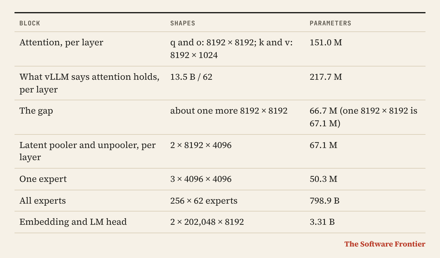
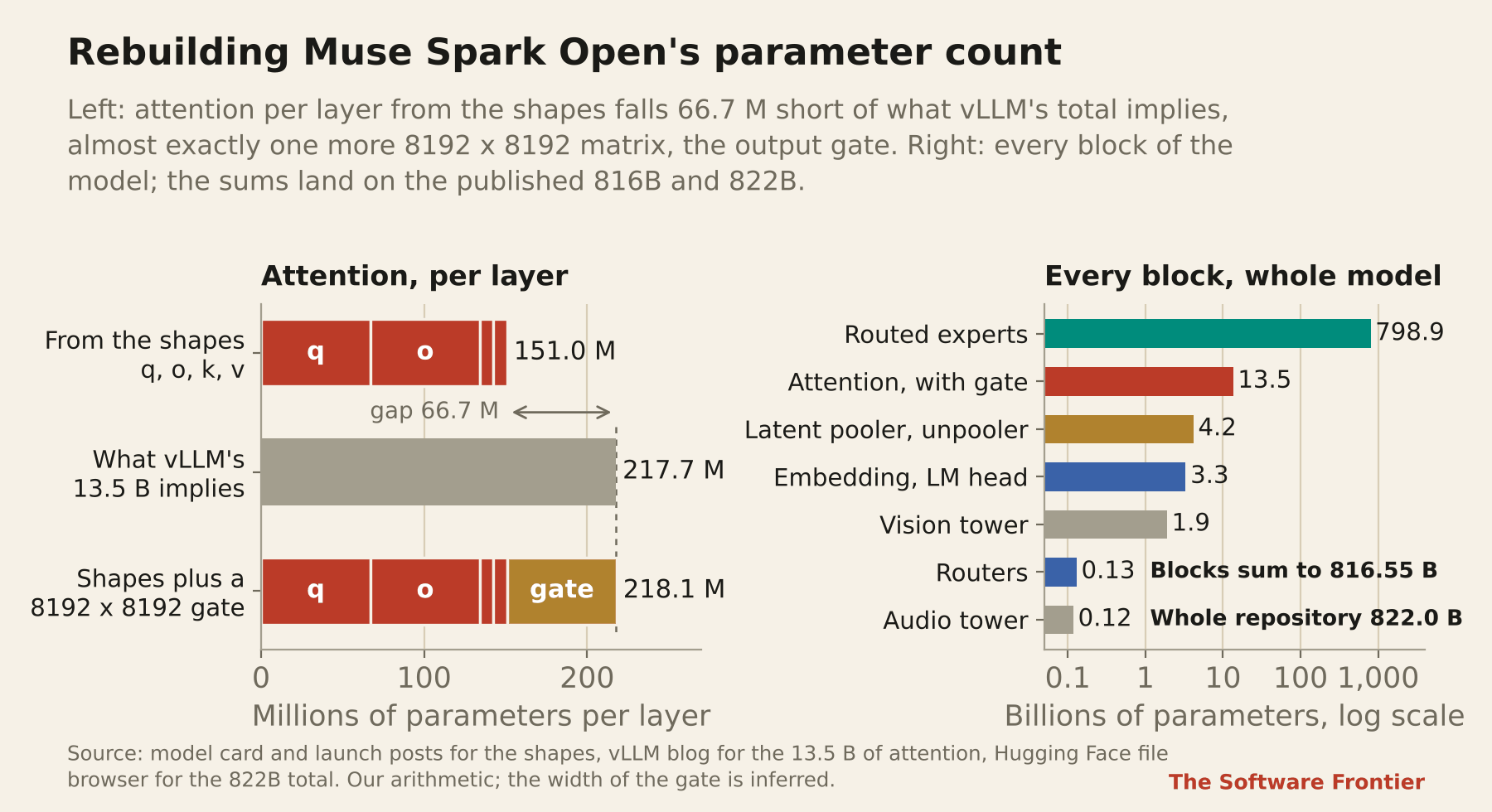
The gap in the third row is the attention output gate, which the card mentions without a size; vLLM’s 13.5 billion is rounded, and a full width gate is the structure that closes it. With the gate, experts plus attention plus latent projections come to 816.55 billion, the headline number.
Adding embeddings, routers and the 1.9 billion vision and 0.118 billion audio towers gives 822.0 billion, which is what Hugging Face displays for the BF16 repository.
The NVFP4 repository is a better test. Hugging Face counts stored elements, so a byte holding two FP4 values counts once and each FP8 block scale counts once per 16 values. The repository displays 484 billion.
The only split that produces that number is FP4 experts in layers 1 to 60 and BF16 everywhere else, including the experts of layers 0 and 61: 386.5 billion packed bytes plus 48.3 billion scales plus 48.9 billion BF16 parameters is 483.8 billion.
The file browser has just told us the quantization recipe, and it agrees with SGLang’s kernel notes and with vLLM’s recipe. A count that does not land is the earliest warning that a later number will be wrong.
Active parameters
Resident parameters set the memory floor. Active parameters set the work per token. For an MoE the two diverge, and the composition of the active set matters more than its size.
Muse Spark Open has 42.65 billion active parameters per token in its blocks: 13.52 billion of attention, 4.16 billion of latent projections and 24.96 billion in 8 of 256 experts per layer, plus 0.13 billion of routers. Attention is 1.7% of what is resident and 31.7% of what is active.
Any reasoning of the kind “it runs like a 42B model” has to say which 42B, because the dense part and the sparse part behave differently under batching and under quantization.
Bytes per step
At low batch, decode speed is set by bytes read per step, so the next number is the active parameters weighted by their storage precision. A checkpoint’s name tells you the precision of its largest tensors, not of the ones you read every token.
For the Muse Spark Open NVFP4 file at batch 1, the routed experts in FP4 are 13.6 GB per token and the BF16 experts of layers 0 and 61 another 1.6 GB, while attention, the latent projections, the LM head and the routers, all BF16, are 38.9 GB. The total is 54.1 GB per output token, and 75% of it is BF16. FP4 covers 94% of the parameters and a quarter of the bytes that set single user latency.
That is why much of the launch day kernel work at NVIDIA, AMD and in SGLang went into BF16 GEMMs, launch overhead and sharding the pooler and unpooler.
KV bytes per token
The fourth number is KV bytes per token of context, and it is the one most often computed wrong. The formula depends on the attention type of each layer:
Global grouped query attention: 2 × KV heads × head dimension × bytes, per layer.
Sliding window: the same, but capped at the window, so it is a fixed cost per sequence rather than a cost per token.
Multi head latent attention: latent rank plus RoPE dimension, times bytes, per layer.
Compressed or shared caches: whatever the report says, because the structure no longer follows from head counts.
Only global and latent layers grow with context, so the number to multiply by is the count of those layers, which lives in layer_types, a sliding window pattern or the model card, never in num_hidden_layers alone. For the open models people serve today, that gives:
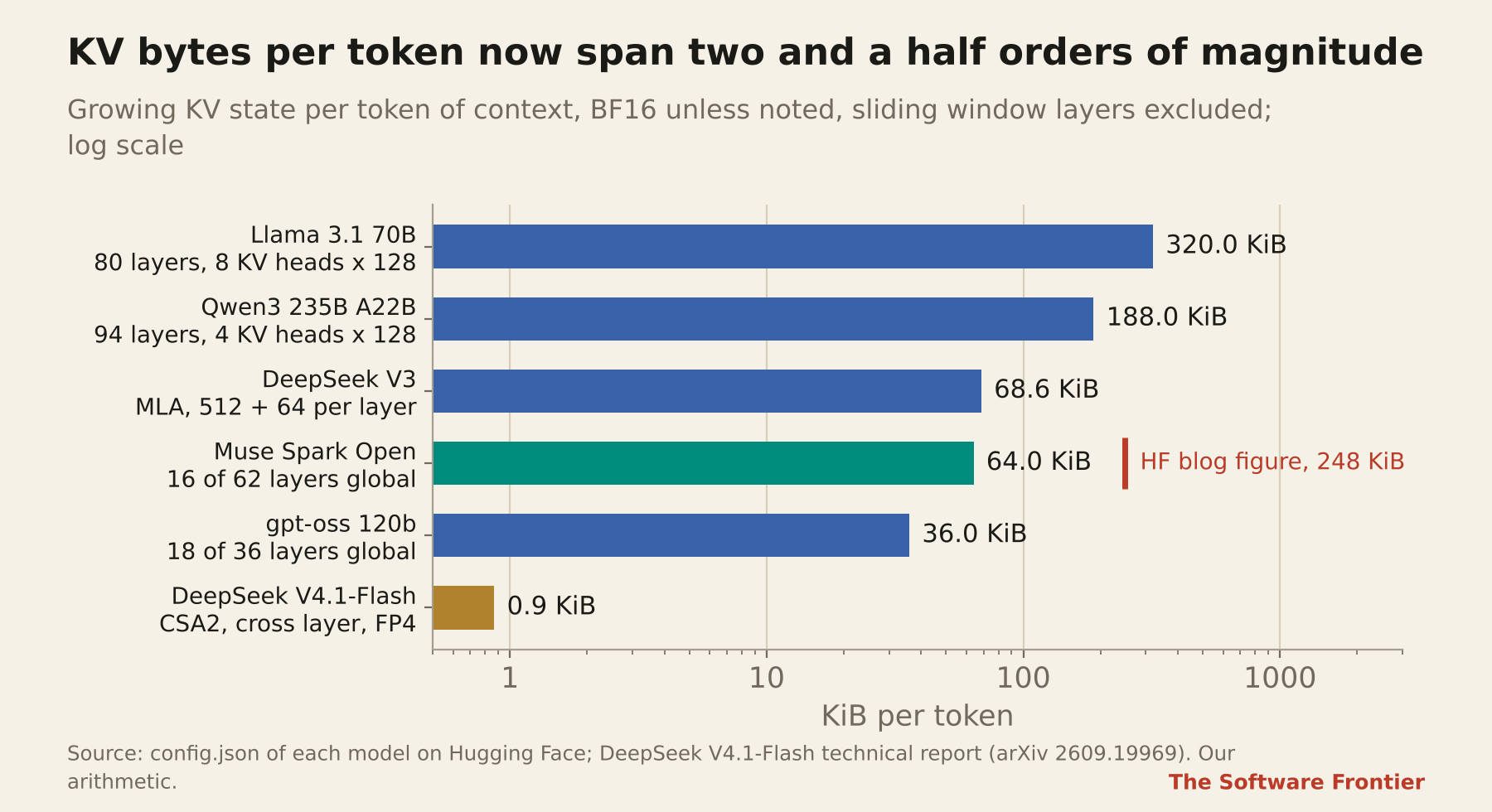
The spread is 368x between Llama 3.1 70B and DeepSeek V4.1-Flash. Two of these models are hybrids whose per token cost is set by a fraction of their layers: gpt-oss 120b alternates 128 token sliding layers with global ones, so 18 of 36 layers count; Muse Spark Open runs three sliding layers to every global one, so 16 of 62 count.
DeepSeek V3 uses latent attention and stores 576 values per layer. DeepSeek V4.1-Flash, which got a new snapshot on October 17, stores 890 bytes in total by compressing the cache, sharing it across layers and keeping it in FP4.
At a million tokens of context these become 68.7 GB for Muse Spark Open’s global layers in BF16 and 0.93 GB for DeepSeek V4.1-Flash. That ratio is a large part of why the two releases are priced so differently.
Expert coverage
Batching amortizes dense weights across sequences. It amortizes expert weights much less, because different tokens pick different experts. If n tokens are routed independently and each picks k of E experts, the expected number of distinct experts read in a layer is
experts touched per layer = E × (1 - (1 - k/E)^n)and the number of tokens needed to read 90% of them is ln(0.1) / ln(1 - k/E). Only the ratio k/E appears. Muse Spark Open (8 of 256), DeepSeek V3 (8 of 256) and gpt-oss 120b (4 of 128) all share k/E = 1/32 and reach 90% at 73 tokens; Qwen3 235B (8 of 128) gets there at 36 and Kimi K2 (8 of 384) at 109.
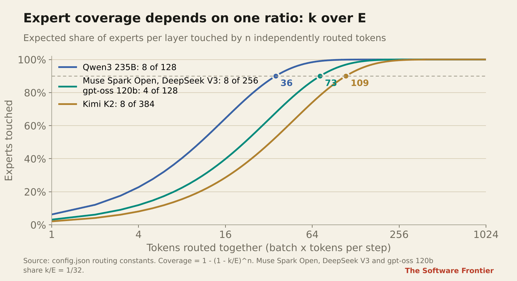
For Muse Spark Open, weight traffic per decode step grows from 54 GB at one token to 477 GB at 73 and 525 GB once every expert is read. The same curve prices speculative decoding and expert parallel load balance, which come up again below.
Real routing is skewed and correlated within a sequence, so these are upper bounds on bytes; they are still the right first estimate.
The attention crossover
Per output token, global attention costs 4 × query heads × head dimension FLOPs per position of context per global layer. Everything else costs about 2 × active parameters, routers included, plus a constant for sliding layers. Setting the two equal gives the crossover, the context length at which attention becomes the larger cost:
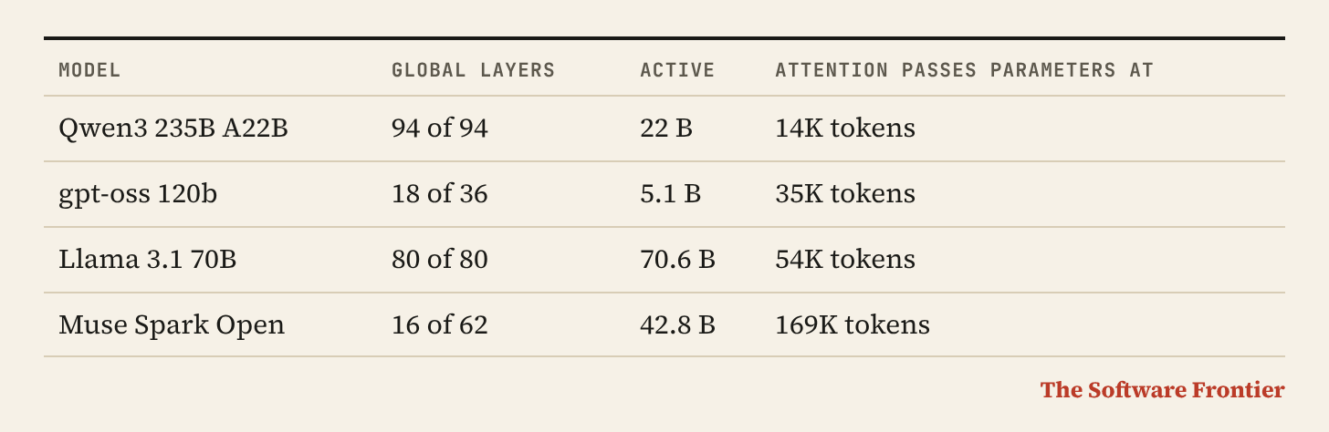
Sparse models with small active sets reach the crossover early, because their parameter cost per token is small while their attention cost is not; Qwen3 235B spends more on attention than on its 22 billion active parameters past 14K tokens.
Muse Spark Open pushes the crossover out by having both a large active set and three quarters of its layers on a window. For prefill the attention sum is quadratic and the crossover doubles: at a million tokens, three quarters of Muse Spark Open’s prefill FLOPs are in its 16 global layers.
Node capacity
The last number is the one that becomes a bill: how many sessions of a given length fit beside the weights. With the NVFP4 weights at 532.7 GB, an FP8 cache and 90% of an HGX B300 node’s 2.1 TB available, 1,357 GB are left for KV.
If every session needed exactly its global cache plus one full window, Muse Spark Open would fit 302 sessions at 128K tokens and 39 at a million. The launch post’s per token figure would have said 10 at a million.
Bytes per generated token then follow from the batch: the shared weights divided by the batch, plus each sequence’s own cache. The weights amortize; the cache does not. At 128K tokens of context the cache alone is 4.49 GB per generated token in FP8, which no batch size removes.
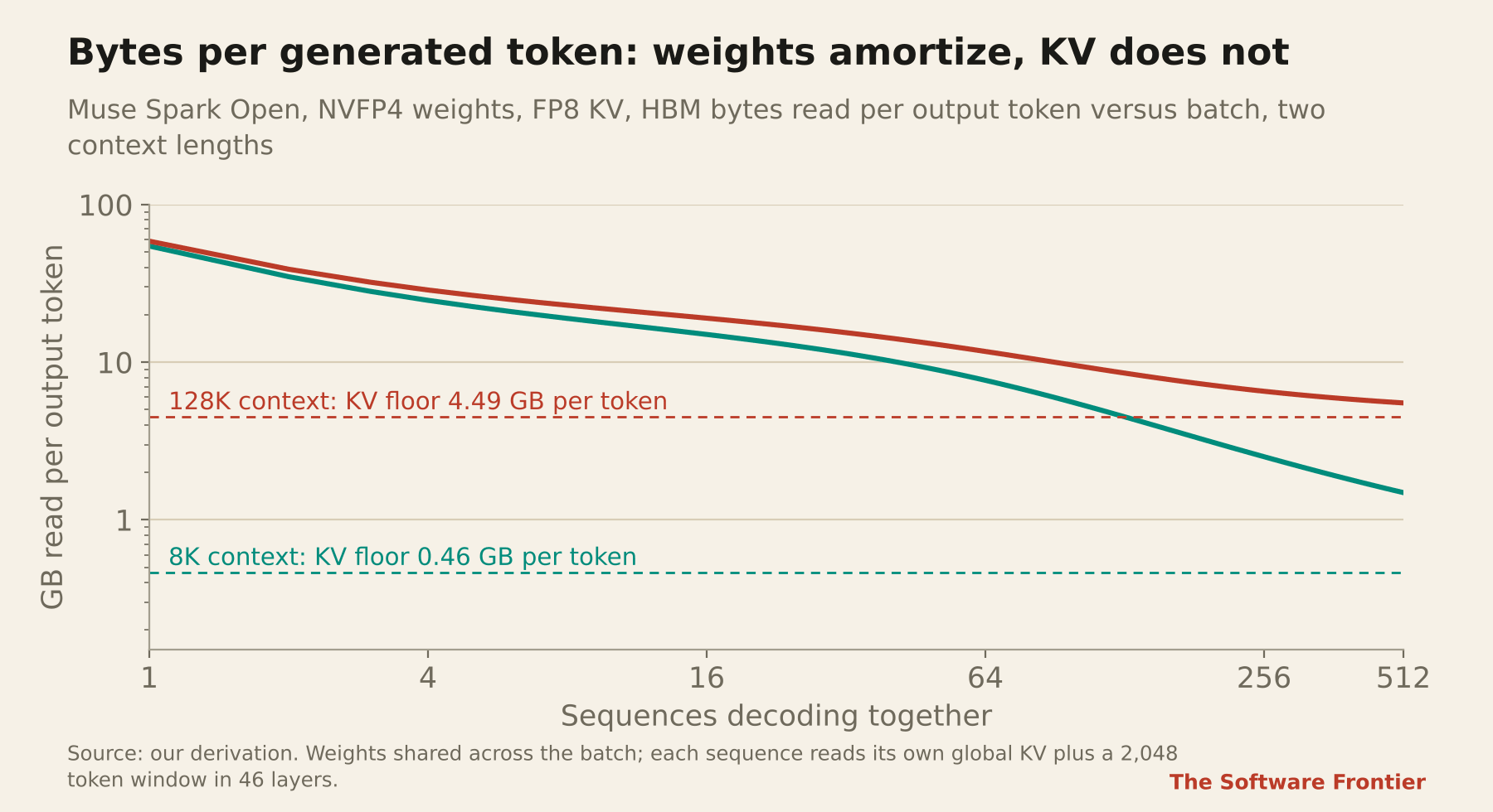
The 302 is a ceiling. What an engine actually fits depends on how it lays out the two kinds of cache, and on how much memory it keeps back for activations, CUDA graphs and a drafter; SGLang’s own GB300 commands keep back 10 to 15%.
Five decisions before launch
The checkpoint
A 4 bit checkpoint’s size follows from its split. NVFP4 stores 4 bit values with one FP8 scale per 16, 4.5 bits or 0.5625 bytes per parameter; MXFP4 uses one 8 bit power of two scale per 32, 4.25 bits or 0.53125 bytes.
With the BF16 tensors that the files keep, that gives 532.7 GB for Meta’s NVFP4 file and 508.5 GB for AMD’s MXFP4 conversion, against 1.644 TB in BF16, and all three match what the recipes list.
Which one to run depends on what the silicon can multiply. Blackwell has FP4 tensor cores for NVFP4 and AMD’s MI350 and MI355 for MXFP4, so on those the 4 bit files run at their native rate and fit a single 8 GPU node with room for cache.
Hopper has neither, so an NVFP4 file on H200 runs through a dequantizing kernel and the memory saving is all you get.
On a Mac the GPU reads the bytes and nothing more, so the format that compresses what every token reads wins: two M5 Ultra Mac Studios at 1.2 TB/s each have a ceiling of 44 tokens per second with the NVFP4 file and 96 with a uniform 4.5 bit quantization of everything.
Keep the BF16 checkpoint for what it is good at, which is producing reference numbers for the accuracy check below.
Parallelism
Tensor parallelism splits every matrix across GPUs and adds two collectives per layer, 124 per token for this model. Expert parallelism places whole experts on GPUs, 32 of 256 per GPU on eight, and replaces those collectives in the MoE block with an all to all exchange.
At low concurrency the exchange carries few tokens and the latency of tensor parallelism is lower; with enough tokens in flight every GPU’s experts are busy and expert parallelism wins.
The published guidance agrees across vendors: plain tensor parallelism for a handful of requests, expert parallelism from about 32 concurrent requests, or from a few when a drafter multiplies the tokens per step. AMD measured 7 to 20% more throughput at 32 to 128 concurrent requests with it.
Whether the exchange can hide behind the expert math has a clean answer, which DeepSeek’s V4 report states as a condition: expert FLOPs per token divided by all to all bytes per token must exceed the GPU’s compute rate divided by its interconnect bandwidth.
For a SwiGLU expert of intermediate size d_ff, each of the k copies of a token does 6 × d_lat × d_ff FLOPs and moves d_lat values out and back, so
FLOPs per byte = 6 × d_ff / (bytes per value sent + bytes per value returned)and the latent width cancels. Muse Spark Open sends NVFP4 with its scales (0.5625 bytes per value) and returns BF16 (2 bytes): 9,591 FLOPs per byte, or 10,961 if one expert in eight is local.
An HGX B300 GPU does 13.5 dense NVFP4 petaFLOPS over 0.9 TB/s of NVLink per direction, which asks for 15,000. The exchange cannot fully hide at peak FP4 rate.
That matters in large prefill batches, and it is one reason part of launch week’s kernel work went into overlapping the exchange with the expert GEMMs.
The memory pools
Engines that support hybrid attention keep one pool for the global layers and one for the sliding layers, and they have to decide how many tokens each holds. In SGLang the decision is --swa-full-tokens-ratio: tokens in the sliding pool divided by tokens in the full pool, default 0.8.
Write F for the bytes a token costs in the full pool and S for the sliding pool. For Muse Spark Open in FP8, F is 16 layers × 2,048 values = 32,768 bytes and S is 46 layers × 2,048 = 94,208 bytes. A ratio r gives the sliding layers a share of the KV memory of
sliding share = r × S / (F + r × S)which at the default is 69.7%. A session of context L needs L tokens in the full pool and at most W + C in the sliding pool, the window plus one prefill chunk. With a KV pool of M bytes the number of sessions is
sessions = min( N / L,  r × N / min(L, W + C) )
where   N = M / (F + r × S)
and it peaks where both limits meet, at r = min(L, W + C) / L. At that ratio every session uses exactly what it needs and nothing is stranded. For 128K sessions with 8,192 token chunks the best ratio is 0.078, which fits 258 sessions on the B300 node, and the default fits 95.
The published values sit in between. On the same node, the 0.4 in the AgentX sweep of SGLang’s launch post fits 146, and the 0.1, 0.15 and 0.2 in the cookbook’s GB300 and MI355X commands fit 245, 220 and 200. As of October 23, the cookbook’s B300 commands and Meta’s deployment guide still leave the default.
The best ratio depends on the context length, and a ratio that is right for one length can be badly wrong for another.
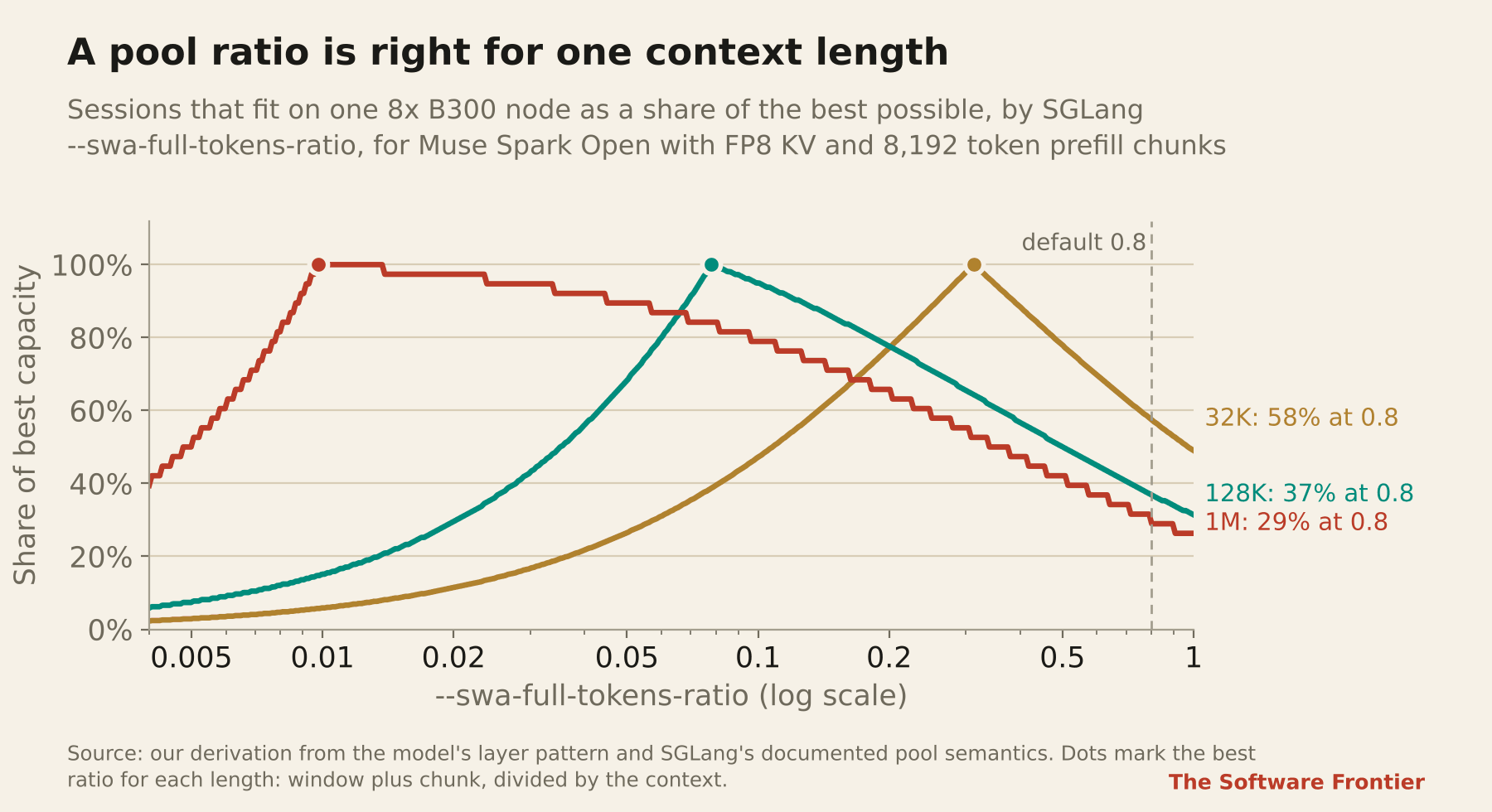
At 32K the best ratio is 0.3125 and fits 665 sessions. The default reaches 58% of that, and 0.1, which is close to right for 128K, reaches only 47%, because the sliding pool runs out before the full one.
At a million tokens the best ratio is 0.0098 and fits 38; the default fits 11. A host that serves one context length should set the ratio for it.
A host that serves a mix has the same balance to strike across every session it holds at once: the sliding pool needs at most W + C per session and the full pool needs each session’s context, so over the sessions held at once
ratio = sum of min(L, W + C) / sum of Lwhich, when every session is longer than W + C, is the window plus one chunk divided by their mean context. A node holding equal numbers of 32K and 128K sessions averages 80K, so the ratio is 0.125, and it fits 370 sessions.
Sized for the long sessions alone, at 0.078, it fits 258, because the short ones run the sliding pool dry; at the default it fits 152. Leave 10 to 20% of headroom on top, so returning agents keep the window state their cached prefix needs.
Two smaller pool decisions go with it. Use an FP8 cache; on GB300, TensorRT-LLM refuses a 16 bit cache for this head dimension when chunked prefill or block reuse is on, and everywhere else FP8 halves the bytes per token.
And size the host memory tier deliberately: SGLang’s --hicache-size is pinned host memory per tensor parallel rank, so Meta’s 200 GB per rank on four GPUs is 800 GB the host must actually have.
Speculative decoding
A drafter proposes a block of tokens and the target model verifies it in one step. On a dense model that step reads the same weights as a plain step, so the gain is close to the acceptance length.
On a fine grained MoE the verify step routes every token in the block, so it reads the experts of B × b tokens instead of B, where B is the number of sequences and b the block size. If the step is bandwidth bound, the gain is the acceptance length divided by how many times more bytes the verify step reads.
For Muse Spark Open with 8 token blocks:
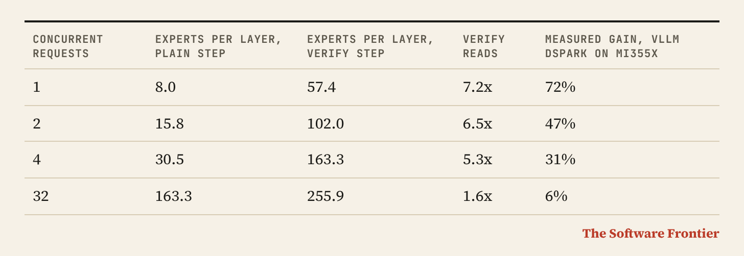
At low concurrency a step is bound by latency, collectives and kernel launches more than by bandwidth, so the extra expert reads are nearly free: in SGLang’s MI355X tables a verify step at 4 concurrent requests takes 1.8 times a plain step while reading 5.3 times the expert bytes.
As concurrency grows the plain step itself starts reading most experts and the verify step has little left to amortize. SGLang’s DFlash V2 on the same hardware fell from 71% faster at 4 requests to 31% at 32. vLLM and AMD both recommend dropping the drafter above about 64 concurrent requests.
The other half of the decision is the acceptance length, which depends on your text. The OpenHands replay fixed it at 4.5 with an environment variable, so its decode speed describes an assumed drafter rather than a measured one.
SGLang’s AgentX sweep measured 4.16 on real coding agent traces. Measure it on your own traffic before you keep the drafter on.
Context and the cache price
The KV cache grows with context and the weights do not, so the cost of an output token grows with the context it is generated in. Filling one B300 node with as many Muse Spark Open sessions as fit and reading the cost per million output tokens at 80% of HBM bandwidth and $6.77 per GPU hour gives $0.44 at 8K, $1.83 at 128K and $13.05 at a million.
The same weights with DeepSeek V4.1-Flash’s 890 byte cache would cost $0.30, $0.34 and $0.60. Somewhere between 256K and 512K, decoding Muse Spark Open costs more than its own list output price. The window exists, but selling all of it at a flat price is a decision, and it is reasonable to cap it at what the business can carry, as Groq’s preview does at 131,072 tokens.
The cache price is the other half of admission. If a host charges p per cached token and holds a session’s cache in a KV pool of M bytes on a node that costs C per second, holding the cache pays for itself as long as the next turn arrives within
T = p × M / (KV bytes per token × C)The context length cancels, apart from the fixed window state, which shortens T slightly at shorter contexts. For Muse Spark Open at $0.15 per million cached tokens on B300s at $6.77 to $9.50 per GPU hour, T is 4.9 to 6.9 minutes at long context, about where the industry’s five minute cache expiry sits.
Spilling idle caches to host memory extends it a long way, because reloading a million token cache over PCIe takes tens of milliseconds.
All of this assumes prefix caching is on. AMD’s day zero vLLM commands turn it off, which is a reasonable choice for a text benchmark and an expensive one for agents: on the SGLang agent replay, every turn would prefill 12.5 times as many tokens.
Three checks before traffic
1. Accuracy against a reference
Quantized MoE kernels fail quietly, so the first check is accuracy against a known reference before anything is served. The SGLang launch post publishes one for this model: GSM8K at 97.80% for the NVFP4 reference on GB300, 97.73% for BF16 and 97.42 to 97.57% for AMD’s MXFP4, with GPQA Diamond between 88.38% and 90.04% across the same configurations.
AMD’s own vLLM runs report GSM8K between 94.4% and 95.5% on MXFP4, about three points lower, which is what a different harness does. Compare within a harness, never across harnesses. Within one, a deployment more than a point below its reference has a kernel or configuration problem, not a quantization problem.
2. The benchmark
The most quoted number from launch week is SGLang’s 80.3K total tokens per second per GPU at 61 tokens per second per user with 128 sessions, on a replay of OpenHands coding agent conversations.
SGLang published the workload, which makes it possible to decompose: 13 turns per conversation, a 74,160 token first turn, 753 new tokens and 220 output tokens per later turn. Per GPU per second that is 73.7K cache hits, 6.4K fresh input and 220 output tokens. Output is 0.27% of the headline.
Per user speed has the same problem. With 128 conversations in flight and 8.0 turns completed per second across the node, Little’s law says each conversation completes a turn every 16.0 seconds. Decoding 220 tokens at 61 per second takes 3.6 of them; the other 12.4 are queueing and prefill. The agent sees 13.8 tokens per second per turn.
A benchmark for day zero should report output tokens per second, turn time and time to first token at the 90th percentile, on traces with the prefix structure and timing of the traffic you expect, with the drafter’s real acceptance and the context length you will admit.
The OpenHands run capped the context at 131,072 tokens and left the pool ratio at its default; neither is wrong for a benchmark, and both matter if you plan from it.
3. Cost per turn
The last check turns the benchmark into money. On the SGLang replay one conversation bills $0.2597 at Muse Spark Open’s list prices of $1.25 per million input tokens, $4.25 output and $0.15 cached: 55.3% from cache reads, 40.0% from fresh input and 4.7% from output.
At 128 sessions a B300 GPU completes 277.2 conversations an hour, so the rental per conversation is $0.024 to $0.034 and the gross margin at list price is 91% to 87%.
With one session per node it is 49% to 28%. The same conversations at DeepSeek V4.1-Flash’s off-peak list prices bill $0.0171, which would not cover the rental even at 128 sessions; at DeepSeek’s peak prices they would roughly break even there.
The formula is short enough to keep next to the benchmark:
margin = 1 - GPU price per hour / (conversations per GPU hour × revenue per conversation)The envelope in code
The arithmetic of the seven numbers and the pool decision fits in one function. It needs only the standard library, and the comments under each call are what it prints.
from math import log, floor

def envelope(c, hbm, gpus, mem_frac=0.9, kv_bytes=1, ctx=131_072, chunk=8_192,
             ratio=None, gpu_hour=6.77, cached_price=0.15):
    """Serving envelope of a GQA + sliding window + MoE decoder, from its config."""
    L, nq, nkv, hd = c["layers"], c["q_heads"], c["kv_heads"], c["head_dim"]
    n_glob = c.get("global_layers", L)                 # count layer_types, not num_hidden_layers
    n_swa, win = L - n_glob, c.get("window", 0)
    E, k = c.get("experts", 1), c.get("top_k", 1)
    per_layer = 2 * nkv * hd * kv_bytes                # K and V, one token, one layer
    full_tok, swa_tok = n_glob * per_layer, n_swa * per_layer
    pool = hbm * mem_frac - c["weight_bytes"]

    # capacity: the architectural ceiling, then what an engine with two pools gets at a ratio
    ceiling = floor(pool / (full_tok * ctx + swa_tok * min(ctx, win)))
    if n_swa:
        swa_need = min(ctx, win + chunk)               # sliding tokens one request can hold
        r = swa_need / ctx if ratio is None else ratio # SGLang --swa-full-tokens-ratio
        n_full = pool / (full_tok + r * swa_tok)
        sessions = min(floor(n_full / ctx), floor(r * n_full / swa_need))
        swa_share = r * swa_tok / (full_tok + r * swa_tok)
    else:
        r, swa_share, sessions = 0.0, 0.0, floor(pool / (full_tok * ctx))

    crossover = (2 * c["active"] + 4 * nq * hd * n_swa * win) / (4 * nq * hd * n_glob)
    n90 = log(0.1) / log(1 - k / E) if E > 1 else 1   # tokens until 90% of experts are read
    node_usd_s = gpus * gpu_hour / 3600
    breakeven_min = cached_price / 1e6 * pool / (full_tok * node_usd_s) / 60
    return dict(kv_bytes_per_token=full_tok, ceiling=ceiling, ratio=round(r, 4),
                swa_share=round(swa_share, 3), sessions=sessions,
                attention_crossover=round(crossover), tokens_to_90pct_experts=round(n90, 1),
                cache_breakeven_min=round(breakeven_min, 1))

muse = dict(layers=62, q_heads=128, kv_heads=16, head_dim=64, global_layers=16, window=2048,
            experts=256, top_k=8, active=42.78e9, weight_bytes=532.7e9)
print(envelope(muse, hbm=2100e9, gpus=8))                 # 8x B300, FP8 cache, tuned pools
# kv_bytes_per_token 32768, ceiling 302, ratio 0.0781, swa_share 0.183, sessions 258,
# attention_crossover 169081, tokens_to_90pct_experts 72.5, cache_breakeven_min 6.9
print(envelope(muse, hbm=2100e9, gpus=8, ratio=0.8))      # the same node at SGLang's default
# ratio 0.8, swa_share 0.697, sessions 95
print(envelope(muse, hbm=2100e9, gpus=8, ctx=1_048_576))  # the full window
# ceiling 39, ratio 0.0098, swa_share 0.027, sessions 38Try it on another model
The calculator below runs the same envelope in your browser. The presets are Muse Spark Open and three open models people serve often; change any field, or type in the constants of a config you are about to deploy.
It also lives on its own page, i used claude to build it, for a simplicity purpose; if you want to keep it open next to a config.
The mistakes these steps catch
Most of what goes wrong in day zero estimates is one of a few patterns, and each step above is there because one of them caught us in our own estimates:
Multiplying by every layer when only some keep a growing cache. Muse Spark Open’s launch post was off by 3.85x.
Leaving an engine’s pool split at its default for a hybrid model. For long Muse Spark Open sessions that is 2.7x fewer sessions on the same node.
Sizing a shared pool for one context length when the node serves a mix. Equal numbers of 32K and 128K sessions fit 370 at the mean context ratio and 258 at the 128K one.
Pricing parameters instead of bytes, as if a checkpoint’s name described all of its tensors. Muse Spark Open’s FP4 file reads 75% BF16 bytes at batch 1.
Treating an MoE as a small dense model when batching it or speculating on it. The expert coverage curve is the difference.
Mixing dense and sparse peak FLOPs, or one part’s compute with another part’s bandwidth. B300’s dense NVFP4 rate is 13.5 petaFLOPS in the HGX version and 15 in GB300; the sparse figures in headlines are higher.
Reading total tokens per second as output, or decode speed as turn time.
Planning from a fixed acceptance length instead of one measured on your text.
Turning prefix caching off for traffic that is 90% cache hits.
Comparing accuracy across harnesses. Three points of GSM8K can come from the harness alone.
Not checking the count. If the rebuilt total does not land on the published one, stop.
Where we might be wrong
Routing is not uniform. The coverage curve assumes every token picks its experts independently and uniformly. Real routers are skewed, and tokens of one sequence tend to pick the same experts, so the byte counts in step 5 and in the speculation table are upper bounds, and the gains we explain with them should come out somewhat better than the arithmetic says.
The pool rule assumes SGLang’s documented semantics. We size each session’s sliding need as the window plus one prefill chunk. If the engine reserves more per request, for speculative tokens or cached branches, every best ratio here is somewhat higher. That 0.8 is far too high for long sessions does not depend on the detail.
Capacity ignores what the engine keeps back. All session counts use 90% of HBM. An engine that keeps back more for activations, CUDA graphs or a drafter fits fewer sessions, in proportion to its smaller KV pool; the best ratios do not change, because they do not depend on the size of the pool.
The exchange condition is a peak rate argument. Expert GEMMs over a few tokens run well below 13.5 petaFLOPS, which makes the all to all easier to hide than the 15,000 FLOPs per byte suggests. The condition says where hiding gets hard, not how fast a given batch runs.
The turn time is a steady state estimate. We derived it from published totals with Little’s law. If the replay put client think time between turns, part of the 12.4 seconds is the client waiting, and the server is faster than our number suggests.
GPU rental moves week to week. We priced B300s from $6.77, the Silicon Data index on October 15, to $9.50, Uvik’s on-demand median. The index read $7.35 on October 22. Every dollar figure here scales with the rental, and the cache break-even shortens in proportion: at $7.35 it is 6.3 minutes instead of 6.9, and the margin at 128 sessions is 90% instead of 91%.
List prices are not contract prices. Large customers pay less and hosts do not run at full utilization, so the margins in the last check are ceilings on what list traffic earns per rented GPU.
LLM Systems Engineering
Since the spring the two of us have been writing a long guide to how LLM inference actually runs, from the GPU up to the invoice. Today we are releasing the free sample here.
It is called LLM Systems Engineering: Inside modern inference, serving and GPU execution pipelines. The October 2026 edition runs to 188 pages: 45 chapters in 11 parts and seven appendices, among them a glossary and a cheat sheet. It is written the way this post is: start from the hardware and the model’s constants, derive the number, then check it against something measured.
What the eleven parts cover, in order:
Foundations. The inference workload, the roofline, the arithmetic intensity of prefill and decode, and the batch size at which decode stops being a memory problem.
GPU-level mechanics. FlashAttention 2 and 3, Flash-Decoding, the KV cache and latent attention, kernel fusion and CUDA Graphs, and what tensor parallel collectives cost.
The engine core. Paged attention, memory pools for hybrid attention models, continuous batching, chunked prefill and prefix caching.
Distributed inference. Prefill and decode disaggregation, speculative decoding, and quantization treated as a memory decision.
Production and failure modes. Tail latency and admission control, why a busy GPU can still be underused, and what each hardware generation changes.
Advanced topics. Expert parallelism, fine-grained experts and the batch sizes at which they stop being cheap, context parallelism, structured output and benchmarking.
Production anatomy. The vLLM V1 process model, observability, agentic and multi-turn workloads, the tokenizer, sampling and the engine ecosystem.
Adapters, storage and streaming. Multi-LoRA serving, the storage hierarchy for KV, what a cached token is worth, and streaming to the client.
Applied systems. Security and multi-tenancy, pipeline parallelism, self-hosting against an API, and Llama 3.1 70B for 1,000 users priced from the step time up.
Beyond dense attention. State space models and hybrids, cross-layer KV sharing and reasoning models.
Field cases and calibration. The method of this post at full length, the Muse Spark Open case, DeepSeek V3 on 96 H100s with its decode step accounted for, and a dated catalog of public measurements from MLPerf v4.1 to v6.0 and SGLang’s H100, GB200 and GB300 series.
This post draws on most of them. The seven numbers are the foundations and the KV cache chapters; the pool, parallelism and speculation decisions come from the engine, distributed and MoE parts; the checks come from the production and benchmark material.
Chapter 42 is this method at full length and Chapter 43 works it through on Muse Spark Open. What the book adds is the detail we had to leave out here, and the cases where the simple formulas stop working.
The appendices hold the parts we use most ourselves: dated hardware, model and price tables in one place, so they can be refreshed as prices and parts change, a cheat sheet of the derivations, and revision notes that list every number that moved since the first edition.
There are 144 numbered references, each of which resolves to a real paper, post or source file. The book ships with derive.py, which recomputes its numbers; run with --verify, it checks 365 printed values and 13 cross-checks and fails if any of them stop agreeing.
We wrote it for engineers who build or operate the serving layer, or who have to make decisions about it: infrastructure and ML platform engineers, people writing kernels or engines, founders sizing a deployment. It assumes you can read Python and know what a GPU is, and it is written around NVIDIA hardware.
We are two people who experiment a lot, read the source and check the arithmetic, and the book is what came out of doing that for a long time.
A free sample with the thesis and all of Part I is linked here, so you can see whether it is for you before buying. If you find a mistake, post it on r/inferencestack; corrections go into the next edition with credit.
Get LLM Systems Engineering The 2026 edition, with the free sample of the thesis and Part I.

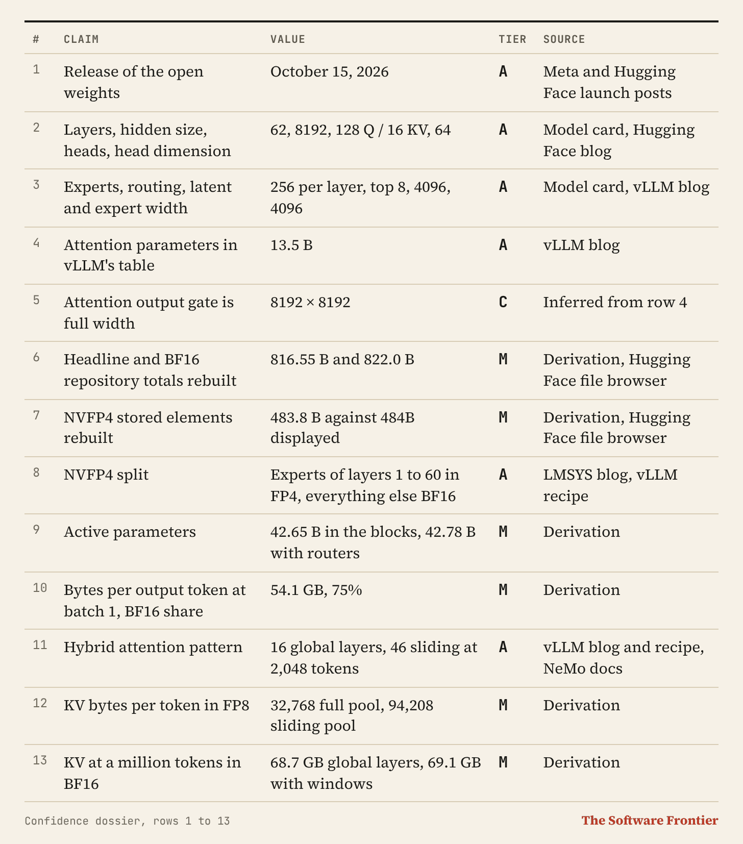
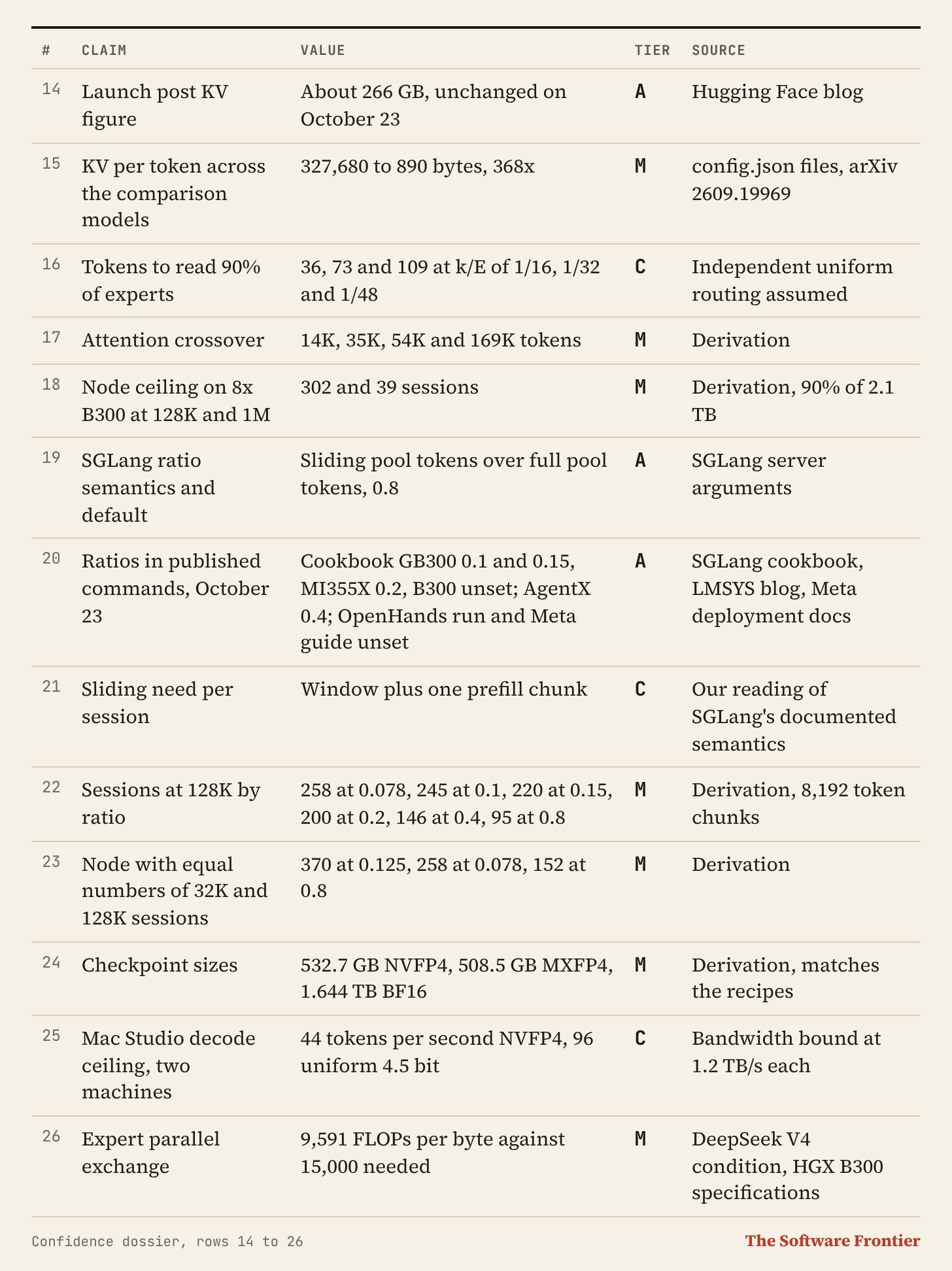
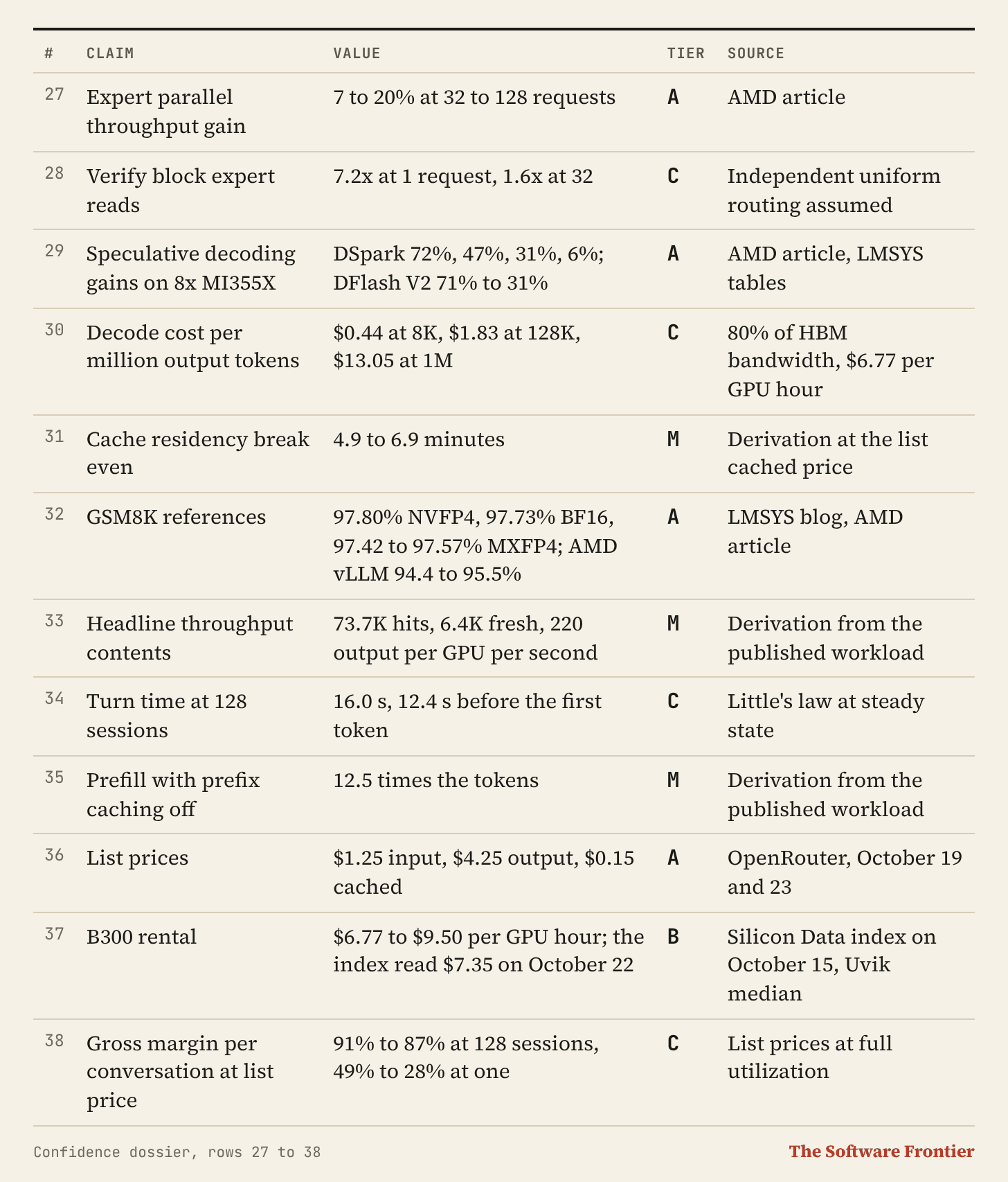
Confidence dossier
Tier A is stated by a primary source. Tier B is stated by a secondary source or by a vendor in marketing material. Tier C is our inference with stated assumptions. Tier D is speculation; nothing in this post needed it. Tier M is our own derivation from published constants, reproducible from the function above and the companion piece.
Sources
Hugging Face, Welcome Muse Spark Open, October 15, 2026, and the model card and file browser for the BF16 repository and its NVFP4 variant.
vLLM Team, Day 0 support for Muse Spark Open on vLLM, October 15, 2026, and the vLLM recipe.
SGLang Team, SGLang and Miles Add Day-0 Support for Muse Spark Open, October 15, 2026; SGLang cookbook, read October 23, 2026; server arguments.
Meta, Build with Muse Spark Open and deployment documentation, October 15, 2026.
AMD, Day 0 Enablement and Optimization for Muse Spark Open on AMD Instinct GPUs, October 2026.
config.json files on Hugging Face for openai/gpt-oss-120b, Qwen/Qwen3-235B-A22B, deepseek-ai/DeepSeek-V3 and meta-llama/Llama-3.1-70B.
DeepSeek-AI, DeepSeek-V4.1-Flash: Pushing the Limits of KV Cache Compression.
OpenRouter, Muse Spark Open and DeepSeek V4.1 Flash 1017, and DeepSeek, Models and pricing, retrieved October 19, 2026; OpenRouter prices checked again on October 23.
Silicon Data B300 Rental Price Index, read October 15 and 22, 2026, and Uvik GPU Price Index, data of October 7, 2026.
Groq, Muse Spark Open model page, preview with a 131,072 token window, read October 23, 2026.
Inference.Engineering, How Muse Spark Open Actually Serves: the long version of every Muse Spark Open number in this post.