



I’ll show you seven numbers this piece derives
284.202 B ; reconstructed backbone against a published 284 B
39.3 % ; of activated parameters are attention, which is 1.74 percent of the weights
3.37 GiB ; of KV for a 1,048,576-token sequence, 1.96 percent of a GQA-8 baseline
79 % ; of attention FLOPs at 1M are the selector, not the attention
4096 ; FLOPs per byte Flash needs from its interconnect, 1.5x Pro’s demand
5,504 ; tokens of recompute restore a million-token prefix, a 191x saving
$2.92 ; per GPU-hour is what 1M context pays; owners clear it, renters do not
I didn’t set out to write about DeepSeek V4-Flash, but i just wanted to check a precise number. The technical report gives the model’s constants in a paragraph on page 25 and its headline size, 284B total and 13B activated, on page 4, and I wanted to know whether the two agreed before I trusted anything else in the document.
They agree to seven hundredths of one percent, but only once you notice that the headline quietly leaves out the multi-token prediction module and that Heavily Compressed Attention carries half the key-value projections that Compressed Sparse Attention does.
Doing the raw math anyway shows something that the report never states: attention is 1.7 percent of this model’s weights and 39 percent of the weights it touches per token.
That is the kind of fact that changes what you build. It means the sparsity everyone is now discussing on reddit, lives entirely in the expert bank, that the attention stack is as dense as it has ever been, and that there is a hard floor under how cheap a model in this family can get. It also doesnt appear in any of the two dozen write-ups of this model I read before starting.
So this is more a reconstruction rather than a summary. Every architectural number below was just rebuilt from the published constants and checked against something DeepSeek or the vLLM team published independently.
Where the reconstruction disagrees with what is currently written about V4-Flash on the open web, I say so. Where it disagrees with the report, I say that too.
What shipped, and what the number on the card means
As of now, there are two DeepSeek-V4-Flash releases and they are the same weights. The preview landed on 24 April 2026 with the 58 page technical report and DeepSeek-V4-Pro.
The official release, tagged 0731, landed on 31 July 2026 as a public beta of the API. DeepSeek’s changelog states that DeepSeek-V4-Flash-0731 has the same model structure and the same size as the preview and that only the post-training was rerun. I’ve not yet seen a new architecture, or a new parameter count; even the price hasn’t changed.
That is convenient for a piece like this, because every architectural fact in the April report still describes the model you can call today. It also means the agent scores DeepSeek published with the 0731 release, Terminal Bench 2.1 at 82.7 and DeepSWE at 54.4, are alignment results rather than efficiency results.
They were measured with DeepSeek’s own harness in what the changelog calls minimal mode at the max reasoning tier, temperature 1.0, top_p 0.95. The harness has not shipped.
Agent scores move by ten points on harness changes. Just treat them as a statement of intent.
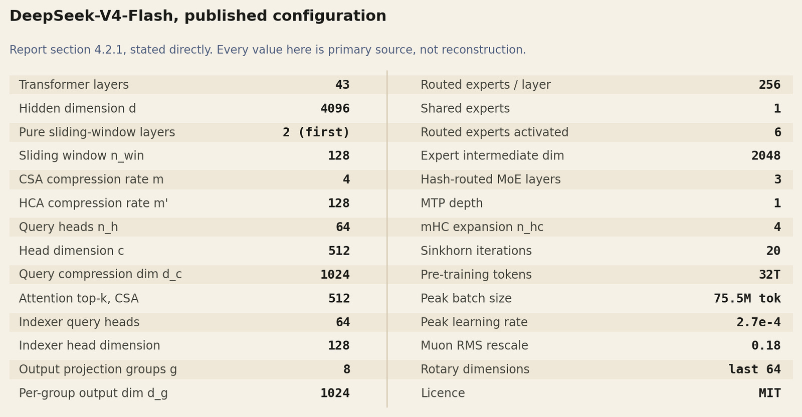
DeepSeek-V4-Flash, published configuration. Report section 4.2.1, stated directly.
I want to focus on one correction, before we go further and deeper. A widely cited third-party guide states that DeepSeek publishes the layer arrangement for Pro but not for Flash, and advises readers to treat Flash’s layer count as unconfirmed.
That is totally wrong. The report gives Flash 43 layers and hidden dimension 4096 in the same paragraph that gives it 284B parameters. Pro gets 61 layers and 7168.
The arrangements differ in one way that matters: Pro’s first two layers are HCA, Flash’s first two are pure sliding window attention with no compression at all.
Rebuilding the model from its constants
Every expert is a SwiGLU block, so three matrices of 4096 by 2048, which is precisely 25.17M parameters. With 256 routed experts plus one shared expert in all 43 blocks, the expert bank alone is 278.108B.
That is 97.8 percent of the model and it takes one line of arithmetic. Everything interesting is (in my opinion) in the remaining 2.2 percent.
The attention shapes are not what you would guess from a normal transformer, and CSA and HCA are not the same size. CSA computes two independent key-value streams, so four projection matrices from equations 9 and 10 of the report.
HCA computes one, so two matrices, from equations 20 and 21. Getting this wrong is the difference between a reconstruction that lands and one that does not.
CSA layer
  W^aKV, W^bKV, W^aZ, W^bZ    4 x (4096 x 512)   =  8.389 M   two overlapped KV streams
  B^a, B^b                     2 x (4 x 512)      =  0.004 M   learnable positional bias
  W^DQ                         4096 x 1024        =  4.194 M   query down-projection
  W^UQ                         1024 x (512 x 64)  = 33.554 M   query up-projection
  W^IUQ                        1024 x (128 x 64)  =  8.389 M   indexer query up-projection
  W^w                          4096 x 64          =  0.262 M   per-head indexer gate
  grouped output, 8 groups     8 x (4096 x 1024)  = 33.554 M
  final output projection      8192 x 4096        = 33.554 M
  attention sink logits        64                 =  0.000 M
                                                    ---------
                                                    121.901 M

HCA layer   one KV stream, no indexer, bias over m’ = 128         109.117 M
SWA layer   uncompressed KV, no compression weights, no indexer   106.954 M
Manifold-constrained hyper-connections add 393K per residual junction. Router gates add 45M across the model. Embeddings, using the DeepSeek-V3 tokenizer with a handful of added context-construction tokens, add 530M on each side.
The report says the vocabulary remains 128K, which I read as the 129,280 entries V3 used.
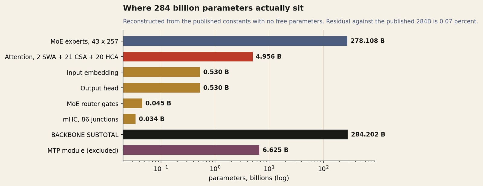
Where 284 billion parameters actually sit. Reconstructed from the published constants; the residual against the published figure is 0.07 percent.
284.202B against a published 284B, a 0.07 percent residual on a reconstruction with no free parameters.
The MTP head is real, it is 6.6B, vLLM will use it for speculative decoding, and it is not in the number on the model card. DeepSeek did the same with V3, whose Hugging Face repository showed 685B against a stated 671B.
There is a second confirmation of the reconstruction hiding in an unlikely place. In the determinism section, discussing why they cannot use split-k for one particular GEMM, the report mentions in passing that “mHC involves a matrix multiplication with an output dimension of only 24.”
With n_hc = 4, the dynamic parameterisation generates A in R^4, B in R^{4x4} and C in R^4 from one flattened input. Four plus sixteen plus four is twenty-four.
The three mappings are produced by a single GEMM, and a throwaway sentence in a section about floating-point associativity confirms the shape.
The activated count follows. Seven experts fire per token, six routed plus the shared one, which is 7.575B. Everything else in the forward pass is dense: all 4.956B of attention, all of mHC, all of the router gates.
That is 12.610B excluding embeddings and 13.140B counting the output head, against a published 13B.
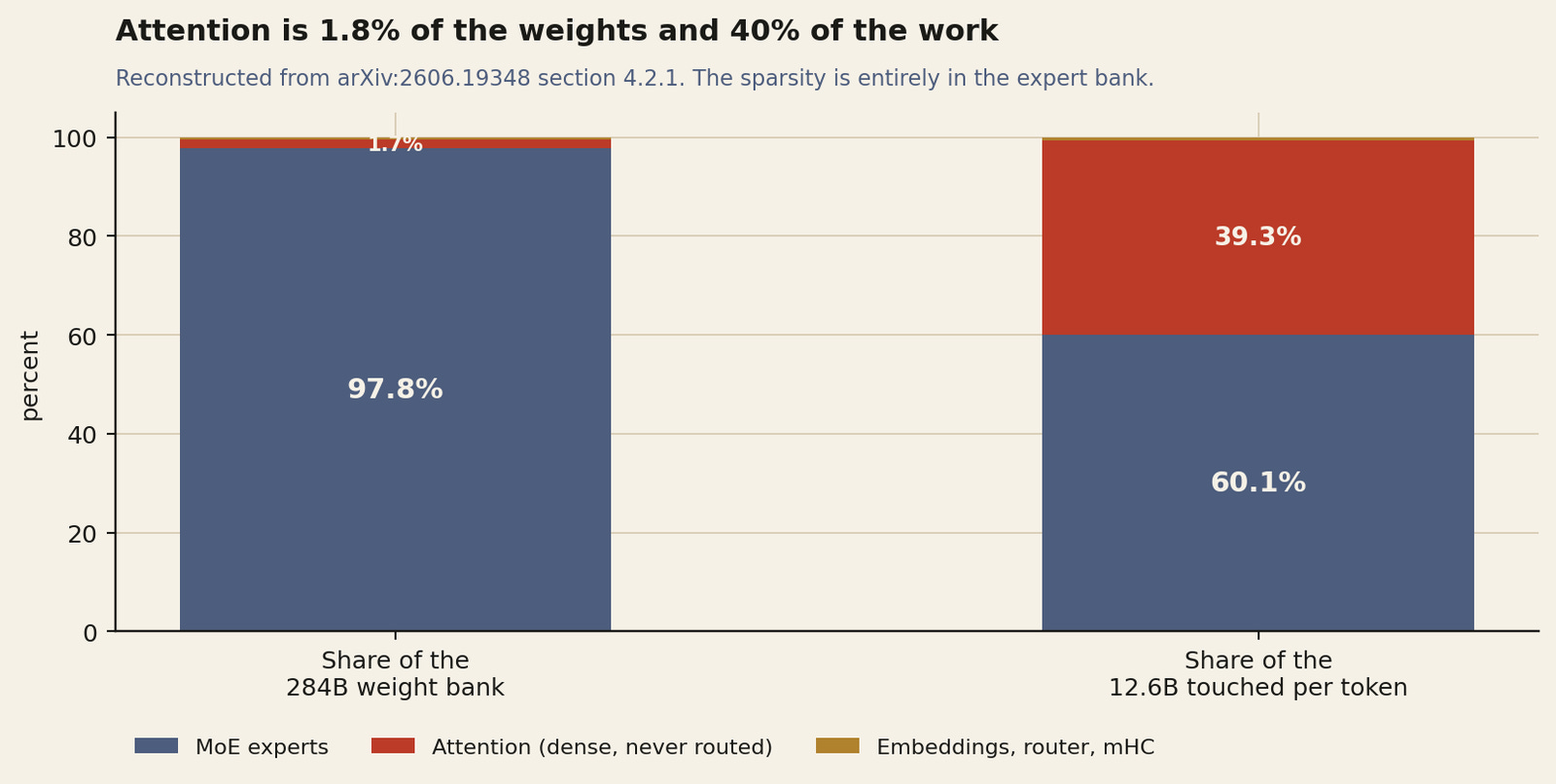
Attention weights are a rounding error in the checkpoint and a plurality of the arithmetic at decode. Reconstructed from the constants in section 4.2.1.
Attention is 1.74 percent of the weight bank and 39.3 percent of what gets touched per token. That’s most load-bearing fact about serving this model and it appears nowhere in the report, because the report presents attention as the thing being optimised away rather than as a fixed cost that survives the optimisation.
The sparsity everyone is discussing lives entirely in the expert bank. The attention stack is as dense as it has ever been.
The consequence is a floor. Push MoE sparsity as far as you like, drop from six routed experts to four, go from 256 experts to 512 at the same activation count, and the activated parameter count will not fall below roughly 5.0B, because the attention stack is dense and it is 4.956B of it.
Every decode step of every request reads all of it. At 12.6B activated you are already 40 percent of the way to that floor. A hypothetical V4-Flash-Nano with two routed experts would be a 10.1B-activated model, not a 4B one.
It also reframes what the hybrid attention is for. It is not there to make attention cheap in absolute terms. It is there to stop attention’s state from growing without bound, which is a memory problem rather than a FLOPs problem, and the FLOPs bill arrives anyway.
We will come back later to how large it gets.
Compressed Sparse Attention
CSA is five separate ideas stacked, and it is often described as one. Taken apart, each of them is simple, and two of them are the sort of thing you only invent after you have been beaten by the alternative.
Key and value are the same vector
V4 stores one cached entry per compressed position, not two. Here, the key and the value are literally the same tensor, used in both roles by a multi-query attention. That is an immediate halving of the cache before any compression happens at all.
It should not work. Attention output is normally translation invariant: rotate the query by R(t) and the key by R(s) and the score depends on R(t-s), which is relative. Values carry no rotation, so the output carries none.
Share the key and the value, and the value inherits the key’s rotation, the output acquires an absolute position through R(s), and shifting the whole sequence changes the answer.
The fix is in section 2.3.3 and it is one line: apply RoPE with position minus i to the last 64 dimensions of each head’s output. Because R is orthogonal and R(t)-1R(s) = R(s-t), rotating the output backwards restores relative positioning, and the contribution of each cached entry ends up depending on its distance from the query again.
The vLLM team’s write-up derives the same result from the other direction and calls it inverse RoPE. Their implementation fuses it into the FP8 quantisation ahead of the output projection, worth two to three times over doing the two separately.
Two times the cache, bought with one elementwise kernel. This is the cheapest trick in the model and it is the one that has attracted the least attention.
The compressor has two streams and they overlap
CSA does not average four tokens into one. It computes two independent projections of the hidden state, Ca and Cb, each with its own learned compression weights Za and Zb, then takes a softmax across the concatenation of 2m weights and forms a weighted sum over both streams.
Compressed entry i draws Ca from positions [mi, m(i+1)] and Cb from positions [m(i-1), mi].
With m = 4 that makes every compressed entry a data-dependent weighted sum of eight consecutive tokens taken at a stride of four. vLLM names this attention type c4a and documents it as a weighted sum of 8 uncompressed tokens with a stride of 4, which is exactly equations 11 and 12.
The overlap is the point. A hard boundary every four tokens cuts arbitrary spans in arbitrary places and the model is blind across the seam. Overlapping means every token appears in two compressed entries under different weights, while the sequence still shrinks by exactly four because the stride is four. The receptive field of an entry is eight; the compression ratio is four.
The compression weights are per dimension. The softmax runs over 2m elements independently for each of the 512 channels, so each channel picks its own mixture of the eight tokens.
This is a learned per-channel pooling rather than a summarisation step, and describing it as “remembering the paragraph’s key point” undersells it by a wide margin.
The Lightning Indexer
After compression a one-million-token context still holds 262,144 entries in every CSA layer. Attending densely to a quarter of a million entries is not obviously better than attending densely to a million, so CSA runs DeepSeek Sparse Attention over the compressed stream: a cheap scoring pass picks the top 512, and the real attention runs only over those.
The scorer builds 64 low-rank query heads of dimension 128 from the same compressed query latent the main attention uses, computes a rectified dot product against a separately compressed indexer key for each block, and sums across heads with a learned per-head gate:
c^Q_t   = h_t · W^DQ                                   shared with the main attention queries
q^I_t   = c^Q_t · W^IUQ                                64 indexer heads of dimension 128
w^I_t   = h_t · W^w                                    one gate per indexer head, from the hidden state
I(t,s)  = sum_h  w^I(t,h) · ReLU( q^I(t,h) · K^IComp_s )
Two choices there are worth stopping on. ReLU rather than softmax leaves the score unnormalised, so a head can contribute nothing to a block rather than merely down-weighting it, and heads can veto. And the gate w is produced from the hidden state by a 4096 by 64 matrix, so the model decides per token which of its 64 scoring heads to trust.
That is a router in everything but name, sitting in front of the attention, and it is trained end to end with it.
Flash’s top-k is 512. Pro’s is 1024. V3.2’s was 2048. The report is direct about the reason: a smaller top-k greatly improves efficiency on short and medium texts, which is where the traffic is.
Grouped output projection
Sixty-four heads at head dimension 512 produce 32,768 values per token. A conventional output projection would be 32,768 by 4096, which is 134M parameters per layer, more than everything else in the attention block put together.
V4 splits the heads into g = 8 groups of eight, projects each group’s 4096 values to 1024, concatenates the eight results into 8192, and projects that to 4096. Total 67.1M, half the naive cost, and the bottleneck at 8192 acts as a constraint on how freely heads can mix.
Pro uses g = 16 at the same d_g = 1024, so a 16,384-wide concatenation from 128 heads. The report also applies RMSNorm per head on the queries and on the single head of the compressed KV entries just before the core attention, which is the same numerical hygiene MLA needed, for the same reason, and which turns out to matter for the optimiser.
Attention sink, and heads that abstain
Both CSA and HCA carry a set of learnable sink logits, one per head. For head h, Exp(z’h) is added to the denominator of the softmax and to nothing else:
s(h,i,j) = Exp(z(h,i,j)) / ( sum_k Exp(z(h,i,k)) + Exp(z’_h) )The report’s description of what this buys is unusually blunt. It allows each query head to make its total attention score not equal to one, “and even to be near 0.” A head with a large sink logit contributes almost nothing to the output no matter what is in the context.
Given that this model asks 64 heads per layer to attend to a top-512 selection out of a quarter of a million compressed blocks, giving heads a principled way to decline is not decoration.
It is what stops a head from being forced to spend its mass on whichever blocks the indexer happened to hand it.
The sliding window is not an optimisation
Every compressed layer also keeps 128 uncompressed tokens in a window, concatenated with the selected compressed entries before the softmax. This is a correctness requirement and the reason is causality.
A compressed entry i in c128a summarises positions 128i through 128(i+1)-1. A query at position t may only use information derived from positions at or before t, so it cannot use entry i unless 128(i+1)-1 is at or before t.
A query sitting anywhere inside the current block therefore has no compressed entry it is permitted to read. Without the window, tokens 1 through 127 of every block would attend to no local context whatsoever.
The window covers the distance between the query and the most recent legal compression boundary, and 128 is exactly m’ for that reason.
Heavily Compressed Attention
HCA is the same compressor at m’ = 128, with two differences that both simplify it. There is one key-value stream instead of two, so no overlap and no seam handling. And there is no indexer, so no top-k. It attends densely over everything it holds.
The arithmetic explains the second choice. A one-million-token context under 128x compression yields 8,192 entries, and eight thousand keys is an ordinary attention problem, shorter than most models’ native context. Sparsity would buy nothing; vLLM implements it as a sparse-attention call with top-k set to 8192, a selection that selects everything, purely so one kernel serves both paths.
Dropping the overlap is defensible because HCA is not responsible for local detail. The sliding window handles that and the interleaved CSA layers handle the middle range. HCA’s job is coarse global memory, and boundary precision on a 128-token block does not matter much when the question is what the document was about.
What the pair produces is a genuinely two-rate memory. In Flash’s stack, two sliding-window layers are followed by 41 alternating layers, giving 21 CSA and 20 HCA.
Every token’s representation passes through 21 layers that can retrieve 512 four-token spans from anywhere in the history and 20 layers that see all 8,192 coarse summaries at once. Neither works alone.
Sparse selection over fine blocks has recall problems on diffuse queries; dense attention over coarse blocks cannot resolve a specific line of code.
The router, and the three ways V4 changed it
Every write-up of this model spends its length on the attention and treats the mixture of experts as inherited furniture. It is not. Section 2.1 makes four changes to routing, and one of them removes a whole class of layer that every DeepSeek model before this one had.
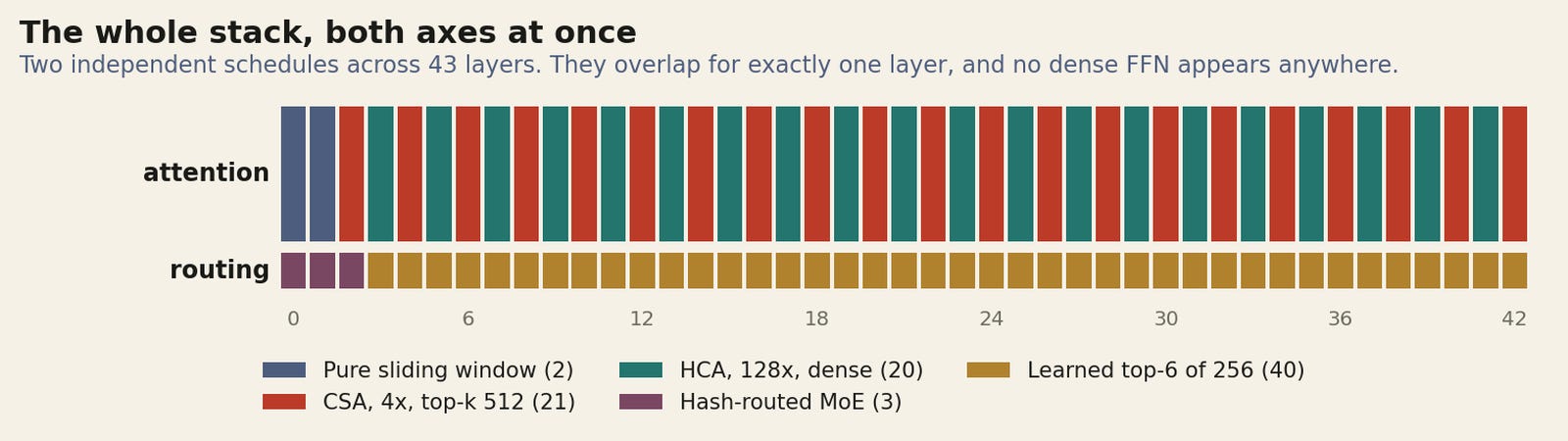
Forty-three layers, two independent schedules. Reconstructed from report sections 2.1 and 4.2.1; the CSA and HCA assignment within the interleave is inferred, and the split is either 21 to 20 or the reverse.
There are no dense FFN layers. V3 kept ordinary dense feed-forward blocks in its first three Transformer layers, on the standard argument that early layers do generic work and routing them wastes capacity.
V4 replaces those with MoE layers that use hash routing: the target experts for a token are fixed by a hash of its token ID, following Roller’s Hash Layers work from 2021. The Hugging Face implementation makes the mechanism concrete.
Routing type is set per layer through mlp_layer_types, and a hash layer resolves its experts through a frozen tid2eid lookup shipped inside the checkpoint.
The details that make this more than a curiosity is that only the selection is static. The learned gate still produces the per-expert scores that weight the chosen experts. So a hash layer is not an un-routed layer; it is a layer where the router has been told which experts to consider and gets to decide how much to trust each one.
That converts the hardest part of early-layer routing, an unstable argmax over 256 options while the model knows nothing, into a fixed assignment with a learnable mixture on top.
It also does something useful for the infrastructure. A hash of the token ID is known before the forward pass reaches the layer, which means dispatch for the first three layers can be planned as soon as the tokens are known rather than after the previous block finishes.
three layers where the overlap is free
The affinity function changed. V3 scored expert affinity with a sigmoid. V4 uses the square root of a softplus. Both are positive and monotone, so the ranking behaviour is similar, but the tails are not. A sigmoid saturates at one, so once an expert is clearly the best its score stops responding and the gradient through it vanishes. Softplus does not saturate, and the square root damps its growth to sublinear without ever flattening. The practical effect is that a strongly preferred expert keeps receiving gradient signal instead of going quiet, which is exactly the failure mode you would expect to precede the routing-driven loss spikes described two sections later.
The routing target cap is gone. V3 constrained how many nodes a token’s experts could be spread across, through the n_group and topk_group parameters, because unconstrained routing means a token’s six experts can live on six different machines and the all-to-all cost is set by the worst case. V4 drops the constraint entirely and says the parallelism strategy was redesigned to pay for it. Which is the same trade appearing again in a different costume. The wave-partitioned mega-kernel in section 3.1 exists so that communication hides under computation. Once it does, capping communication to protect throughput stops being necessary, and the model gets its routing freedom back. Every efficiency result in this report buys an architectural freedom somewhere else, and the report never quite says so.
Load balancing stays auxiliary-loss-free, with one addition. V4 keeps V3’s scheme, where a per-expert bias is added to the score for the purpose of top-k selection and excluded from the gating weight, so balance is enforced without a gradient term competing with the language modelling objective. The Hugging Face implementation keeps it as an e_score_correction_bias buffer that shifts the argmax without carrying gradients. On top of that V4 adds a mild sequence-wise balance loss whose only job is to stop a single sequence collapsing onto a handful of experts, with a weight of 0.0001 and a bias update speed of 0.001. Global balance from a bias, local balance from a loss, and the loss is small enough to be a guardrail rather than an objective.
Manifold-Constrained Hyper-Connections
Hyper-connections widen the residual stream from one vector to n_hc vectors and let the model learn the mixing, which decouples residual width from hidden size.
The update is Xl+1 = BlXl + ClFl(AlXl), with A projecting the widened stream down to the layer input, C projecting the layer output back up, and B mixing the residual lanes among themselves.
DeepSeek’s stated problem with plain hyper-connections is that stacking them is numerically unstable. B is applied at every junction, so across 86 junctions the model computes a product of 86 learned matrices. If the spectral norm of B exceeds 1 by any margin, the product diverges. If it falls below 1, the signal dies.
The fix is to constrain B to the Birkhoff polytope, the set of doubly stochastic matrices: nonnegative, every row and column summing to one. Two properties make this the right set rather than a convenient one.
A doubly stochastic matrix has spectral norm exactly 1, so the residual mapping is non-expansive by construction and neither the forward nor the backward pass can blow up through it. And the set is closed under multiplication, so a product of 86 of them is still doubly stochastic. The stability is structura-l, not empirical.
Projection onto the polytope uses Sinkhorn-Knopp: exponentiate the raw matrix for positivity, then alternate row and column normalisation, twenty times. A and C get a sigmoid, with C scaled by two so it can express amplification up to a factor of two while staying nonnegative, which rules out lanes cancelling one another.
One implementation detail worth recording because the paper skips it: the widened stream has to collapse before the output. A final hyper-head folds the four residual lanes back into a single sequence just ahead of the model norm, so the language modelling head sees an ordinary hidden state and nothing downstream needs to know the residual was ever four vectors wide.
At n_hc = 4 this costs 393K parameters per junction and 34M across the model, about a hundredth of one percent of the weights. The cost is elsewhere. The residual stream is four times wider in activation memory, twenty Sinkhorn iterations sit on the critical path of every junction, and pipeline communication between stages grows.
DeepSeek’s answer is obviously fused kernels, a recomputation strategy that checkpoints most inter-layer hidden states and all normalised layer inputs while leaving compute-intensive operations alone, and an adjustment to the DualPipe 1F1B overlap so parts of mHC run concurrently with the pipeline.
The number they report for the whole apparatus is 6.7 percent of the overlapped 1F1B stage.
SGLang found the other end of the same problem at serving time. In low-latency decode the batch is small, the pre-GEMM that feeds the Sinkhorn normalisation has almost no parallelism, and it becomes the bottleneck. Their answer was to split the K dimension of that GEMM across CTAs.
Which is where the determinism section’s remark about an output dimension of 24 comes from: the GEMM is small enough that split-k is compulsory and split-k is non-deterministic, so they emit each split separately and reduce in a following kernel.
Muon, and the thing it did not break
V4 trains with Muon for most parameters and AdamW for the embedding, the prediction head, the static biases and gating factors of mHC, and all RMSNorm weights. Momentum 0.95, weight decay 0.1, update RMS rescaled to 0.18 so the AdamW learning rate schedule could be reused unchanged.
The orthogonalisation is a hybrid Newton-Schulz, ten iterations in two stages. The first eight use coefficients (3.4445, -4.7750, 2.0315), which converge fast and overshoot; the final two use (2, -1.5, 0.5), which are gentler and settle the singular values precisely at one.
Splitting the schedule this way is the practical answer to a known tension in Newton-Schulz: aggressive coefficients reach the neighbourhood quickly and oscillate there, conservative ones land cleanly but slowly.
The detail worth flagging is a negative result. Muon has a documented pathology where orthogonalised updates keep singular values near uniform, query and key norms drift up together, and pre-softmax logits reach values low precision cannot hold. Moonshot’s answer in the Kimi work was QK-Clip.
DeepSeek states plainly that they do not use it, because the attention architecture already applies RMSNorm to the queries and the KV entries, which prevents the logits from exploding in the first place.
So the RMSNorm in section 2.3.3, which reads like routine hygiene, is load-bearing for the optimiser choice. That is a co-design decision presented as a footnote.
How the sparsity was actually taught
You can’t train a top-k selector from scratch. If the indexer is random at initialisation, the attention sees 512 random blocks, the gradient signal for choosing better blocks is buried, and the model learns to ignore the compressed path entirely.
The schedule in section 4.2.2 solves this in stages, and it is worth reading as a recipe rather than a list. Flash starts at sequence length 4K and extends through 16K and 64K to 1M. Attention is dense for the first 1T tokens. Sparse attention is introduced at the 64K stage, and before it is switched on there is a short stage that warms up the lightning indexer alone. Then sparse attention runs for the rest of training, which is most of 32T tokens.
The ordering is the interesting part. Dense first so the model learns what to attend to; then an indexer warmup so the selector learns to imitate the dense attention’s choices; then sparsity, at a sequence length long enough that selection matters and short enough that dense supervision was still affordable to produce.
Pro gets a longer dense stage than Flash, which is what you would expect if the dense phase is the expensive part and the larger model needs more of it.
Two other schedule details are worth having. Batch size ramps to 75.5M tokens and stays there. Learning rate warms over 2000 steps to 2.7e-4, holds, then decays to 2.7e-5 on a cosine near the end.
MTP loss weight is 0.3 for most of training and drops to 0.1 when the learning rate starts decaying, which reads as a decision to stop letting the speculative head pull on the backbone once the model is being finished.
The instability, and the two things that fixed it
The report is unusually candid here. Training was unstable, rollbacks did not prevent recurrence, and the spikes were consistently traced to outliers in the MoE layers, with the routing mechanism itself appearing to make the outliers worse.
Two techniques fixed it and DeepSeek says openly that they do not have a theory for why.
Anticipatory routing. It decouples the routing decision from the backbone update. At step t the model computes features with current parameters but routes with parameters from step t minus delta, and to avoid loading weights twice they fetch step t’s data early and cache the routing indices during the earlier step’s forward pass. That costs about 20 percent of wall time, so they do not run it continuously: an automatic detector triggers a short rollback and switches the mode on when a spike occurs, then reverts after a period. Amortised, the overhead is close to nothing. The mechanism is worth thinking about. If routing and features update together, a token that starts going to a bad expert gets a gradient that makes both the expert worse and the routing decision more confident, which is a positive feedback loop with no damping. Freezing the routing for a few steps breaks the loop by making the router a fixed target that the experts have to fit rather than a moving one that co-adapts.
SwiGLU clamping is the blunt half. The linear component is clamped to [-10, 10] and the gate component is capped at 10, throughout the training of both models. Clamping an activation is what you reach for after watching a run diverge, and DeepSeek reports it eliminates outliers without compromising performance.
What the cache costs, checked four ways
The report gives ratios against DeepSeek-V3.2 and vLLM gives absolute figures for Pro. Nobody publishes the absolute figure for Flash. It is derivable, and the derivation can be validated before it is used.
Build a byte model from the published dimensions. Section 2.3.3 fixes the rotary dimension at exactly 64, and section 2.3.4 specifies bf16 for the RoPE dimensions and FP8 for the rest, so a shared key-value entry of head dimension 512 costs 64 times 2 plus 448, which is 576 bytes.
The indexer cache runs in FP4 under quantization-aware training, so a 128-dimension indexer key costs 64 bytes.
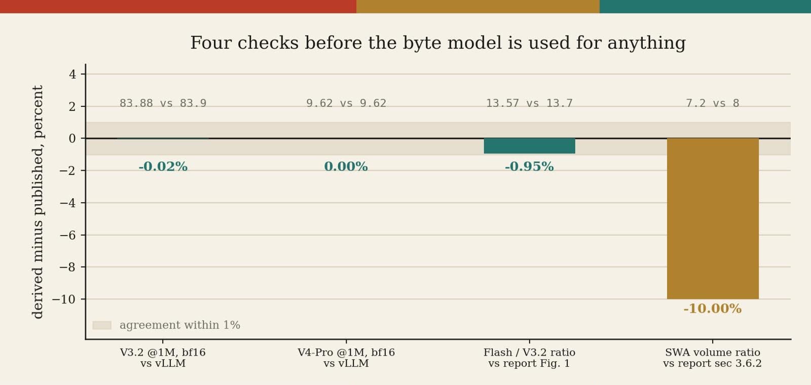
Two against figures vLLM published independently, two against ratios stated in the report itself.
V3.2 caches an MLA latent of 512 dimensions plus 64 RoPE and a 128-dimension indexer key. In bf16 that is 1,408 bytes per token per layer, which over 61 layers at 1,048,576 tokens is 83.88 GiB. vLLM publishes 83.9. V4 at Pro’s 30 CSA and 31 HCA layers gives 9.62 GiB in bf16. vLLM publishes 9.62. Applying the same model at production precision, V3.2 comes to 49.12 GB and Flash to 3.62 GB, a ratio of 13.57 to one, against the 13.7x the report prints on Figure 1.
And section 3.6.2 says the uncompressed sliding-window state would be roughly eight times the volume of the compressed state; the byte model says 7.2.
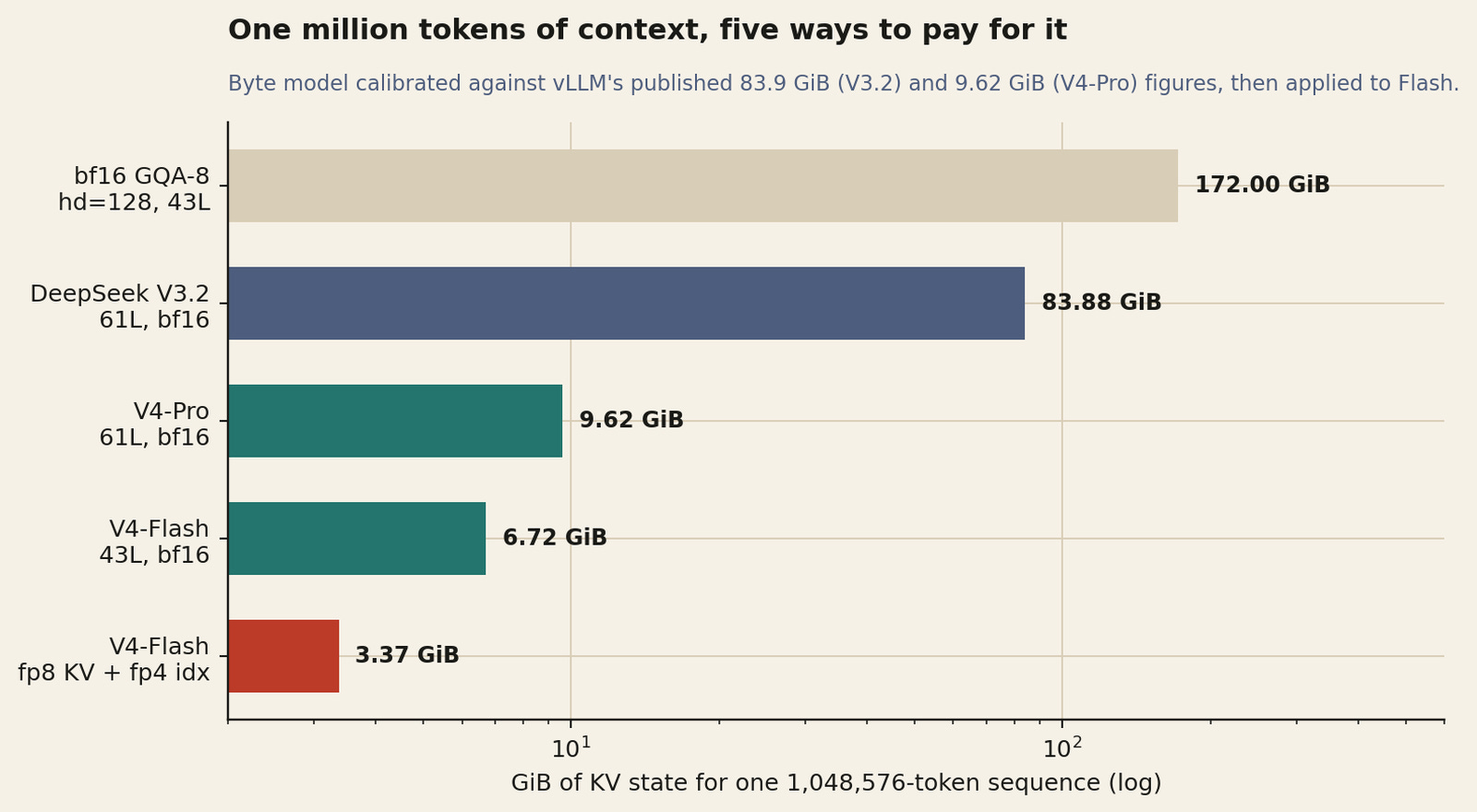
One 1,048,576-token sequence. The model reproduces vLLM’s published V3.2 and V4-Pro figures before being applied to Flash.
So: 3.372 GiB per one-million-token sequence, or 3,453 bytes for each token of context across the whole 43-layer stack. Against the baseline the report chooses, bf16 grouped-query attention with 8 KV heads at head dimension 128, which is 176,128 bytes per token and 172 GiB for the same sequence, Flash comes in at 1.96 percent.
The report claims approximately 2 percent. Derived independently, it holds.
Three multipliers produce that and only one of them is the headline. Fifty-one times from sequence-axis compression and the interleave, two times from sharing key and value, and slightly under two times from mixed FP8 and FP4 storage.
Top-k selection, the mechanism everyone names when they describe this model, saves no memory at all. It saves bandwidth at read time. The memory win is compression, sharing and precision, in that order.
The indexer is O(n), and that is the ceiling
Here is what the efficiency section does not say. Top-k selection bounds the cost of attending. It does not bound the cost of selecting. To pick the best 512 of 262,144 compressed entries, the indexer scores all of them. That scan is linear in context length and it never becomes sparse.
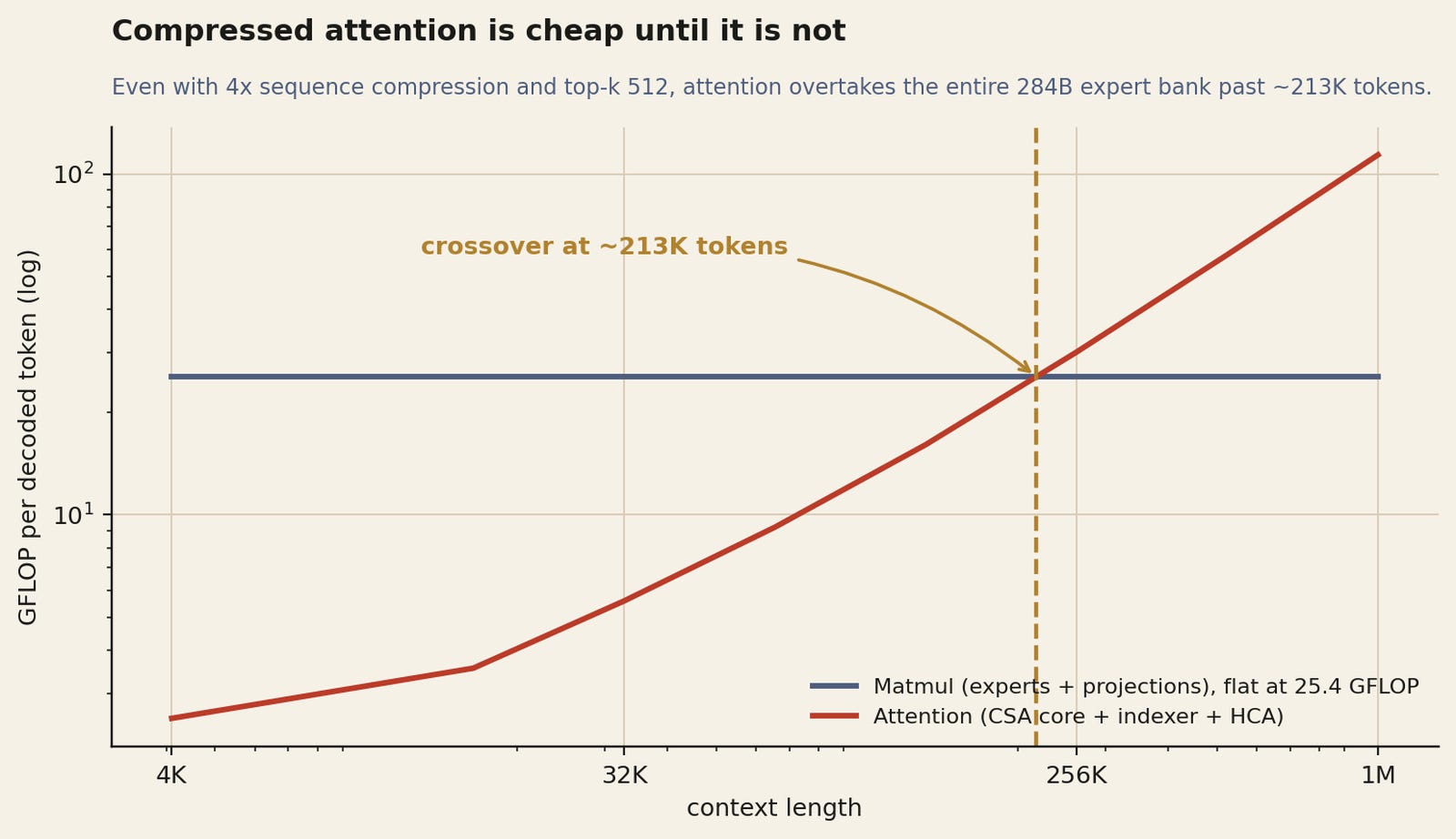
The matmul side is flat by construction. The attention side is linear in context because of the indexer scan and the HCA dense pass.
At 4K of context, attention is 9 percent of per-token arithmetic and the model behaves like a cheap 13B. At 32K it is 18 percent. At 128K it is 39 percent. Around 213K tokens the attention overtakes the entire 284B expert bank, and at 1M it is 82 percent of the work.
The model is linear in context, not sub-linear. Compression changed the constant by roughly fifty. It did not change the exponent.
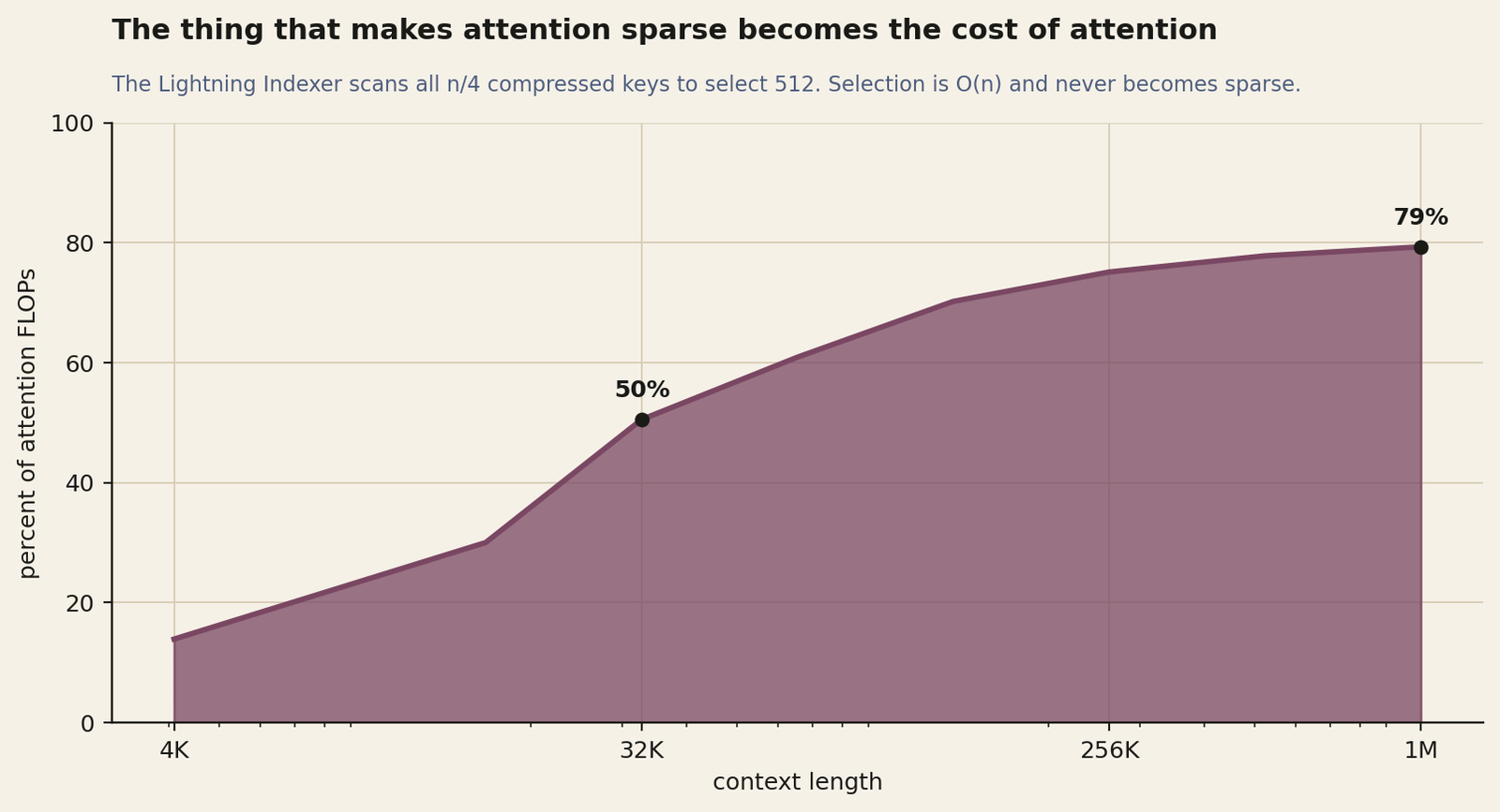
At 32K of context, half the attention arithmetic is spent deciding what to attend to. At 1M, four fifths of it is.
Half the attention FLOPs at 32K are the indexer. Four fifths at 1M. The thing that makes attention sparse is the dominant cost of the attention.
Four fifths of the cost of attention in this model is the cost of deciding what to attend to.Derived from the published dimensions
DeepSeek clearly knew. The indexer runs in FP4 while the main attention runs in FP8, which is the more aggressive precision going to the larger consumer. Flash’s top-k came down to 512 while Pro’s is 1024, because reducing k shrinks the attention pass and does nothing at all to the scan, and Flash needs the attention pass small relative to its smaller matmul side.
And the compression rate m = 4 is not primarily a memory optimisation: the scan runs over n/m keys, so compressing by four is a four times discount on selection, with the cache saving arriving as a side effect.
If someone finds a sub-linear selector, this architecture gets a second life. There is already a paper trying, from a group that fine-tuned V4-Flash with a Neural Memory Indexer that predicts and prefetches only the query-critical KV chunks, reporting comparable benchmark scores at 13.5 percent of the GPU memory.
Its authors are explicit that the work was constrained by resources and cut short, with the indexer trained on frozen keys and no end-to-end optimisation against the backbone. As a result it is a direction rather than a result. It is the right direction.
FP4, down to the index scores
The so-called Quantization-aware training is applied during post-training to two things: the MoE expert weights, and the query-key path of the CSA indexer, where activations are cached, loaded and multiplied entirely in FP4.
The expert-weight scheme has a property worth stating because it explains why the whole thing was affordable. Master weights are held in FP32, quantised to MXFP4, then dequantised back to FP8 for the actual computation, and the FP4 to FP8 dequantisation is lossless.
FP8 in E4M3 has two more exponent bits than FP4 in E2M1, so as long as the ratio between the largest and smallest scale factors of the FP4 sub-blocks, which are 1 by 32 tiles, inside a given FP8 quantisation block, which is 128 by 128, stays under a threshold, the finer scale information is absorbed entirely by the wider dynamic range.
DeepSeek verified their weights satisfy the condition. The consequence is that the entire QAT pipeline reuses the existing FP8 training framework without modification, with a straight-through estimator carrying gradients back to the FP32 masters, and no need to requantise transposed weights.
Then there is one number in that section that deserves its own paragraph. They also quantise the index scores themselves, the output of the lightning indexer, from FP32 to BF16.
That gives a two times speedup on the top-k selector while preserving a 99.7 percent recall rate of KV entries. Given that the selector is the dominant term in attention cost at long context, halving it for three tenths of a percent of recall is the highest-leverage line in the report.
During rollouts and any inference-only forward pass, including teachers and reference models, real FP4 weights are used rather than simulated quantisation, so sampling behaviour during RL is identical to deployment behaviour.
That is a correctness argument dressed as an efficiency one, and it matters: a policy trained against a simulated-quantisation rollout is optimising a model that will never be served.
The mega-kernel, and the balance point DeepSeek wants hardware to hit
Expert parallelism needs an all-to-all dispatch and an all-to-all combine per MoE layer, and the conventional implementation runs communication and computation as separate serial kernels, which leaves both the interconnect and the SMs idle half the time.
DeepSeek’s answer fuses them into one pipelined kernel and then partitions the experts into waves. As soon as every expert in a wave has its tokens, that wave computes, while the next wave’s tokens are still in flight and the previous wave’s results are being sent back. In steady state all three proceed at once.
The reported gains are 1.50 to 1.73 times against strong non-fused baselines for general inference, and up to 1.96 times for latency-sensitive work like RL rollouts and high-speed agent serving, where batches are small and long-tailed and the pipeline has the most idle time to recover.
The report’s own figure puts the theoretical ceiling of the wave scheme at 1.92 times against 1.42 for Comet, which overlaps dispatch with the first linear and the second linear with combine but not at wave granularity, and it evaluates both in the V4-Flash configuration specifically. The implementation is open, as MegaMoE inside DeepGEMM, and it was validated on both NVIDIA GPUs and Huawei Ascend NPUs.
Then comes the paragraph I think is the most economically consequential in the entire report, and it is addressed to hardware vendors rather than to users.
Communication hides under computation when C/B is at most Vcomp/Vcomm, where C is peak compute and B is interconnect bandwidth. For a DeepSeekMoE layer each token-expert pair costs 6hdff FLOPs across the gate, up and down projections, and 3h bytes of traffic, being h bytes of FP8 dispatch and 2h bytes of BF16 combine.
The h cancels. The condition collapses to:
C / B <= 2 * d_ffThe report evaluates this for Pro, whose expert intermediate dimension is 3072, and gets 6144 FLOPs per byte, then observes that once bandwidth clears that threshold it stops being the bottleneck and further silicon spent on it brings diminishing returns. Their recommendation to hardware designers is to target the balance point rather than scale bandwidth unconditionally.
The report contains the equation that says the cheaper model is the harder one to host. It does not evaluate it for the cheaper model.Report section 3.1
Flash’s expert intermediate dimension is 2048. Run the same derivation and Flash’s balance point is 4096 FLOPs per byte, which is two thirds of Pro’s.
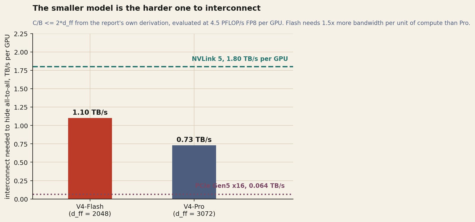
Derived from the report’s own condition at 4.5 PFLOP/s of dense FP8 per GPU. Smaller experts do less arithmetic per byte moved.
The smaller model is the harder one to interconnect. Flash needs 1.5 times more bandwidth per unit of compute than Pro does, because its experts do less arithmetic for the same number of bytes dispatched and combined.
At a B200’s dense FP8 throughput, Flash wants about 1.10 TB/s per GPU to hide its all-to-all and Pro wants about 0.73. NVLink 5 covers both comfortably. A PCIe Gen5 box does not cover either, and misses Flash by a factor of seventeen.
Anyone sizing a deployment on the assumption that the cheaper model is the easier one to host has the relationship backwards, and the report contains the equation that says so.
Three other proposals in that section are worth recording because they are a roadmap. DeepSeek asks for more power headroom, on the grounds that extreme fusion drives compute, memory and network to high load simultaneously and power throttling becomes the limiter, which is a real and underdiscussed consequence of fusing everything.
They use pull-based communication, where each GPU reads from remote GPUs, because fine-grained push carries too much notification latency, and they ask for lower-latency cross-GPU signalling so push becomes viable.
And they propose replacing SwiGLU with a cheap elementwise activation with no exponential and no division, because that lightens post-GEMM work and, under a fixed parameter budget, removing the gate projection lets dff grow, which pushes the balance point up and relaxes the bandwidth requirement further.
That last one is a description of the next model.
TileLang, and a theorem prover in the compiler
Section 3.2 is the part of this report that a compiler person should read twice. DeepSeek’s architecture, written naively, decomposes into hundreds of fine-grained Torch ATen operators, and they replaced most of them with fused kernels written in TileLang, a tile-level DSL, rather than in CUDA.
They did two things to TileLang along the way are more interesting than the choice itself.
Host codegen. As accelerators get faster, CPU-side orchestration becomes the ceiling for small kernels, and the usual source is host-side logic such as runtime contract checks written in Python for flexibility. DeepSeek co-generates the device kernel and a lightweight host launcher at the IR level, embedding data types, rank and shape constraints and stride and layout assumptions parsed from the frontend, then lowers the launcher to host source on TVM-FFI, whose compact calling convention and zero-copy tensor interop keep the overhead small. Validation and argument marshalling happen in generated C rather than in Python. Their measurement: CPU-side validation drops from tens or hundreds of microseconds per invocation to under one.
That is a two-order-of-magnitude reduction in a cost that most people do not measure at all, and it is the sort of thing that only shows up when your model has enough small kernels for launch overhead to dominate. Which this one does, by construction.
Z3 in the algebraic system. TileLang kernels are full of complex tensor index arithmetic, and passes like layout inference, memory hazard detection and bound analysis all need to prove properties of integer expressions before they are allowed to fire. Weak integer reasoning means conservative passes means slower kernels. DeepSeek integrated the Z3 SMT solver into TileLang’s algebraic system, translating integer expressions into quantifier-free non-linear integer arithmetic, which handles the ordinary linear index algebra through ILP and the harder cases, such as vectorising over variable tensor shapes, through genuine non-linear reasoning. They report a few seconds of added compilation time and improvements across vectorisation, barrier insertion and simplification.
A production LLM shipped with an SMT solver inside its kernel compiler. This is the direction I have argued the field goes: the bottleneck in kernel performance is not the language, it is how much the compiler can prove, and buying proving power off the shelf is cheaper than hand-writing the kernel.
The numerics policy in the same section is equally deliberate. Fast-math is disabled at the compiler level by default, precision-affecting approximations are opt-in frontend operators, and IEEE-compliant intrinsics with explicit rounding modes are available when strict semantics are required.
They also align TileLang’s algebraic simplification and lowering rules with NVCC so that kernels can be validated bit-for-bit against hand-written CUDA baselines, with layout annotations available to pin down lowering decisions and hold accumulation order constant. Accuracy by default, speed by opt-in, which is the opposite of the usual arrangement.
Bitwise batch invariance, and why they wanted it
Batch invariance means a given token’s output is bitwise identical regardless of where it sits in a batch. Almost nobody ships this, because it costs performance, and DeepSeek’s reasoning for paying is that they wanted bitwise alignment across pre-training, post-training and inference, which makes loss spikes diagnosable and post-training behaviour consistent with what gets served.
Getting it required giving up two standard optimisations and then engineering the loss back out.
Attention. Split-KV, which spreads one sequence’s attention across many SMs to balance load, is not batch invariant. Abandoning it causes wave quantisation, where the final partially filled wave of thread blocks leaves most of the GPU idle. DeepSeek’s answer is a dual-kernel decode: a first kernel computes an entire sequence’s attention inside a single SM, giving throughput on fully occupied waves, and a second kernel spreads one sequence across multiple SMs to shorten the trailing partial wave. The two are engineered to have the same accumulation order so their outputs are bit-identical, and the second uses distributed shared memory within thread-block clusters to exchange partial results across SMs at speed. The reported overhead of batch-invariant decoding after this is negligible.
Matrix multiplication. cuBLAS cannot be made batch invariant, so it is replaced end to end by DeepGEMM. Split-k, which is how you get performance at very small batch, is also not batch invariant, so it is dropped in most scenarios and the resulting loss is recovered by other means.
Determinism is a separate problem from batch invariance and it comes from accumulation order, usually via atomic addition in the backward pass.
Sparse attention backward normally uses atomicAdd to accumulate KV gradients, so they allocate a separate accumulation buffer per SM and do a global deterministic summation afterwards. MoE backward is non-deterministic because SMs from different ranks negotiate write positions into the same receiving buffer, so they pre-process token order within each rank and isolate buffers across ranks.
And the mHC GEMM with its output dimension of 24 is small enough that split-k is unavoidable, so each split is emitted separately and reduced deterministically in a following kernel.
There is a payoff for this that shows up two sections later, in the rollout service. Because generation can be preempted at any time on their cluster, they keep a token-granular write-ahead log per request and resume from it.
The report explains why they cannot simply regenerate interrupted requests from scratch, and the argument is a good one: shorter responses are more likely to survive an interruption, so regenerating the survivors biases the training distribution towards short outputs.
They note that a batch-invariant deterministic stack could fix this instead by regenerating with a consistent sampler seed, but that this still costs a full re-decode, so the log wins. Batch invariance is what makes that alternative even expressible.
Two cache hierarchies, and lcm(4, 128)
The hybrid attention breaks the assumption PagedAttention is built on, which is that every layer’s KV state has the same shape and the same eviction policy.
In V4 the compression ratios differ per layer, the indexer carries its own embedding size, the sliding-window layers have their own hit and eviction rules, and there is a rolling residual of tokens not yet numerous enough to compress that has to live somewhere.
DeepSeek splits it in two. A classical paged KV cache holds the compressed CSA and HCA entries. A separate state cache holds the sliding-window entries and the uncompressed tail, on the argument that both are a function only of the current position, which makes them a state-space model rather than a growing history, so a fixed-size pool can be pre-allocated and assigned per sequence.
The block geometry falls out of the two compression rates. A block has to cover a whole number of compressed entries in every layer, so it must span a multiple of the least common multiple of m and m’.
For Flash that is lcm(4, 128) = 128 original tokens, giving 32 CSA entries and exactly one HCA entry per block. vLLM independently chose 256 native positions, which is two of DeepSeek’s minimum blocks, giving 64 c4a entries and 2 c128a entries.
vLLM’s implementation notes are the best serving document published on this model, and their three decisions are worth having next to DeepSeek’s.
One logical block size in native token positions for every compressed layer, so slot mapping, scheduler accounting and prefix-hit detection use one unit instead of branching on the compression ratio. The compressor’s rolling residual registered as sliding-window KV with sliding_window set to the compression stride, rather than as a side buffer, so prefix caching lands on block boundaries and disaggregated prefill ships it through the existing SWA transfer path instead of a second one.
And a page-size argument: page size is block_size times compress_ratio times entry_size, all three are controllable, and chosen carefully the five cache kinds collapse into three buckets, each backed by one pool, sized once at load, with no runtime repartitioning and no cross-kind fragmentation.
On the kernel side vLLM fuses three groups: compressor with RMSNorm, RoPE and cache insertion, all elementwise, for 1.4 to 3 times; inverse RoPE with FP8 quantisation ahead of the output projection, for 2 to 3 times; and a horizontal fusion of query normalisation, KV RoPE and sliding-window key insertion using static warp-ID dispatch, each warp working independently on a query head or a key head with no cross-warp communication, for 10 to 20 times over the naive version.
The indexer then runs on its own CUDA stream alongside KV compression and window insertion, worth 5 to 6 percent end to end at low batch.
SGLang went at the FP4 weights instead, pairing MXFP8 activations with MXFP4 expert weights through FlashInfer’s TRTLLM-Gen fused MoE backend, and splitting K across CTAs in the mHC pre-GEMM for exactly the small-batch parallelism problem described earlier.
What a cache hit actually costs
DeepSeek stores all compressed CSA and HCA entries to disk.
When a request hits a stored prefix, those entries are read back rather than recomputed, up to the last complete compression block; the tail of an incomplete block still has to be recomputed because uncompressed entries are not stored.
The sliding-window state is the problem. It is uncompressed and it exists in every layer, so storing it for every token would be roughly eight times the volume of everything else.
The report gives precisely three strategies with different trade-offs, and the third is the one that makes the economics work.
Full SWA caching stores everything, so a hit reads the last n_win tokens of the prefix and recomputes nothing. Zero redundancy, but only a sliver of what was written is ever read, which is a write-heavy unbalanced access pattern that SSDs handle badly.
Periodic checkpointing saves the window state every p tokens, loads the nearest checkpoint on a hit and recomputes the tail, with p tuning the storage against compute trade.
Zero SWA caching stores none of it. Here is the argument, and it is the neatest piece of reasoning in the report. Each token’s sliding-window entry in a given layer depends only on the window entries of the previous layer, which span n_win tokens. So the dependency cone going back through L layers is exactly n_win times L tokens wide. Recompute that many tokens and the entire window state is restored.
A million-token prefix comes back for the price of five and a half thousand.Report section 3.6.2, zero SWA caching
For Flash, n_win times L is 128 times 43, which is 5,504 tokens. Restoring the full sliding-window state of a one-million-token prefix costs a 5,504-token recompute, about 140 TFLOP, against the 26.6 PFLOP a cold prefill of that prefix would cost. That is a factor of 191, and it is why a cache hit can be sold for a fiftieth of a cache miss.
The whole thing only works because the compressed state is small. Storing 172 GiB per session on disk is possible, but reading it back at request time competes with the prefill it was meant to replace. At 3.62 GB it does not.
Compressing the sequence axis is what turns disk from a bad idea into the cheapest tier in the hierarchy, and the $0.0028 line on the rate card is the direct commercial expression of that.
Post-training, and the parts of it that are cost mechanisms
The pipeline broadly follows DeepSeek-V3.2 with one substitution the report calls critical: the mixed reinforcement learning stage is replaced entirely by on-policy distillation.
Domain specialists are trained separately, each through supervised fine-tuning then GRPO against domain-specific rewards, and then more than ten of them are merged into one student by having the student sample its own trajectories and minimise reverse KL against the relevant teacher.
They use full-vocabulary logit distillation rather than the usual token-level KL estimate, on the grounds that the cheap estimator has high gradient variance and destabilises training. Making that affordable took two tricks.
Teacher weights live in centralised distributed storage and are loaded on demand with ZeRO-like sharding.
And rather than materialising logits for a vocabulary above 100k across more than ten teachers, they cache only the last-layer teacher hidden states and reconstruct logits on the fly through the prediction head at training time, ordering training samples by teacher index so exactly one teacher head is resident on device at a time. The KL itself is a TileLang kernel.
Three things from the post-training section have direct consequences for what you pay.
The reasoning ladder is a context ladder
Three modes, trained as separate RL configurations with distinct length penalties and context windows, then unified. Non-think evaluates at 8K of context, Think High at 128K, Think Max at 384K. Non-think emits an empty reasoning block and goes straight to the summary.
Think Max additionally prepends a system instruction, printed verbatim in the report, which tells the model that shortcuts are not permitted and that it must document every intermediate step, considered alternative and rejected hypothesis.
That instruction is why Artificial Analysis measures this model generating 210M output tokens across its index against a 100M median. The verbosity is not a training accident.
It is an instruction, in the system prompt, that DeepSeek wrote and that you are billed for at $0.28 per million. Anyone running Flash at max effort and complaining about token burn is paying for a behaviour they asked for by name.
The tool schema is XML on purpose
V4 introduces a tool-call format built on a dedicated |DSML| token with XML-shaped invocations rather than JSON.
String parameters go through as-is with an explicit string=”true” flag; everything else is JSON-encoded with the flag false. The stated reason is that XML mitigates escaping failures and reduces tool-call errors.
This is a small decision with a large downstream effect. Every escaping failure in a JSON tool call is a wasted turn, and a wasted turn in an agent loop costs a full round of prefill plus decode. Reducing tool-call error rate is a cost reduction that never appears on a rate card.
Interleaved thinking, and a warning inside it
V3.2 kept reasoning traces across tool-result rounds but discarded them when a new user message arrived. V4 keeps everything, across user message boundaries, for tool-calling conversations, so a long-horizon agent maintains one cumulative chain of thought instead of reconstructing its state each turn.
General conversation keeps the old discarding behaviour, on the reasonable grounds that persistent traces buy little there and cost context.
The warning is in the same paragraph and it is easy to miss. Agent frameworks that simulate tool interactions through user messages, and the report names Terminus, will not trigger the tool-calling context path and therefore will not get the persistence.
DeepSeek’s own recommendation for those frameworks is to use non-think models. If you are benchmarking Flash inside a harness that fakes tools as user turns, you are measuring the wrong path.
Quick Instruction, which is an inference-economics feature wearing a post-training costume
In a chat product, a handful of auxiliary decisions run before the real response: whether to trigger a web search, what the query should be, how authoritative a source needs to be, what domain the request belongs to, whether a pasted URL should be fetched.
The standard answer is a separate small model, which means a second prefill of the same prompt because it cannot share the big model’s KV cache.
DeepSeek trained special tokens for each of those tasks and appends them to the input sequence directly. The auxiliary task runs on the already-computed KV cache. There is no second prefill, several of the tasks run in parallel, the user-perceived time to first token drops, and there is no small model to maintain.
The published tokens are |action|, |title|, |query|, |authority|, |domain|, |extracted_url| and |read_url|. Read the list and it is obvious this is DeepSeek’s own chat product spilling into the model card, which is exactly what makes it interesting.
It is a vertical integration of the router into the weights, and it deletes a whole class of serving infrastructure that everyone else runs.
The sandbox, briefly
Agentic RL needs somewhere to execute, and DeepSeek built a platform they call DSec: three Rust components on top of their 3FS distributed filesystem, running hundreds of thousands of concurrent sandbox instances per cluster.
One Python SDK abstracts four execution substrates behind one API, switchable by a parameter.
Function Call dispatches stateless invocations to a pre-warmed pool with no cold start.
Container is Docker-compatible with EROFS on-demand image loading. MicroVM is Firecracker for security-sensitive high-density work.
FullVM is QEMU for arbitrary guest operating systems.
Base images sit on 3FS as read-only layers shared across instances, writes go to a local copy-on-write layer, and snapshots chain, which gets them millisecond-scale resumption.
Each sandbox keeps a globally ordered trajectory log of every command and result, which serves three purposes: fast-forwarding after a preemption by replaying cached results rather than re-executing non-idempotent commands, provenance for every state change, and deterministic replay of any historical session.
None of this is in the model. All of it is why the model has agent scores.

What a node holds
Now the economics, and they start with capacity rather than speed.
Four B200 at 180 GB usable is 720 GB of HBM. The weights ship natively mixed: FP4 for routed experts, FP8 for attention, norms and router. That is 139 GB plus 6 GB, call it 145 GB resident.
At 85 percent HBM utilisation, leaving room for activations, the four-times-wider mHC residual stream and the compressor states, the KV pool is roughly 467 GB.
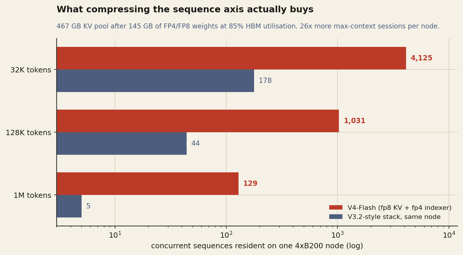
The same node, the same money, the same power draw. The difference is which axis was compressed.
129 concurrent one-million-token sessions on one four-GPU node. A V3.2-style stack on the same hardware holds five. At 128K, the working length of most real agent traffic, it is 1,031.
This is the actual product. Not the million-token window as a marketing number, but the ability to keep a thousand long-lived agent sessions warm on one node without evicting anyone.
Eviction is what makes long-context serving expensive, because every eviction is a re-prefill and a re-prefill of 128K tokens costs more than the entire conversation that followed it. Compressing the sequence axis turns that from a scheduling problem into a non-problem.
The roofline, and what $0.28 buys
Decode on a large MoE is bandwidth-bound. At any batch deep enough to hit every expert, the node streams the full expert bank once per step: 278.1B parameters at FP4 is 139 GB, plus the dense stack replicated across four data-parallel ranks, giving 164 GB of weight traffic per step against 32 TB/s of aggregate bandwidth. A 5.12 ms floor, or 195 steps per second.
Artificial Analysis measures 122.7 output tokens per second per user on DeepSeek’s own API, which is 8.15 ms per step. The model achieves 63 percent of peak HBM bandwidth. That is a good number for something with this much elementwise work between matmuls, and it is a direct vindication of the fusion work in both vLLM and DeepSeek’s own kernels.
Holding that efficiency and adding KV read traffic gives node throughput, and node throughput times $0.28 per million gives revenue.
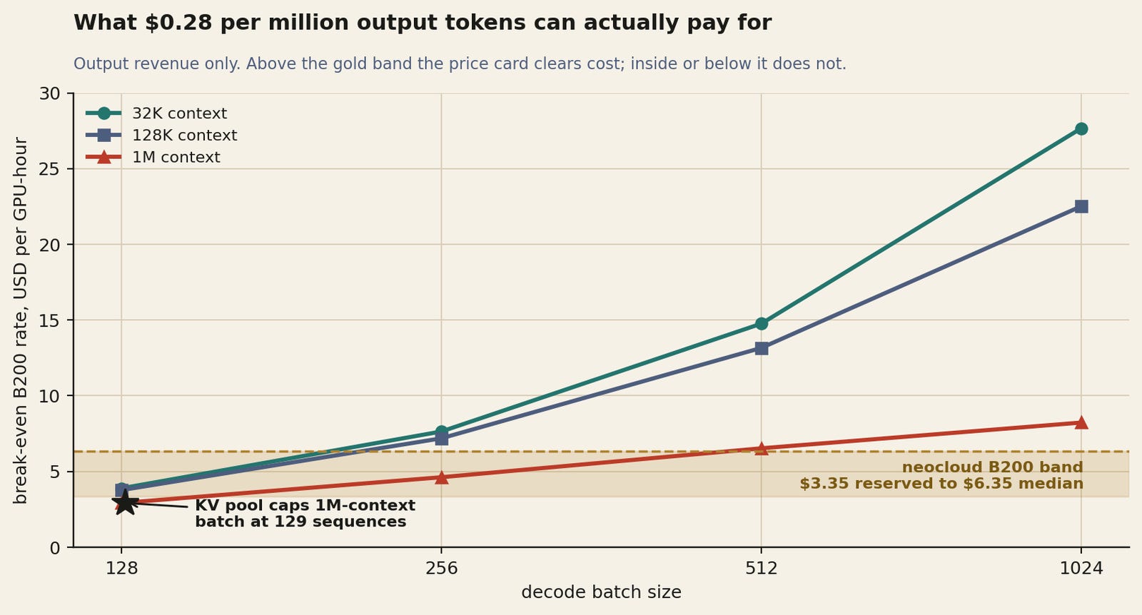
Break-even GPU rate from output revenue alone. The gold band is the rentable B200 market, roughly $3.35 reserved to $6.35 median as of August 2026.
At 32K of context you need a sustained decode batch of about 256 before $0.28 per million covers a mid-market B200 at $5.50 per GPU-hour. At 512 you clear 57 percent gross margin, at 1024 you clear 77.
At 1M of context it never clears: the KV pool caps the batch at 129 sequences and the break-even rate there is $2.92 per GPU-hour, below the cheapest reserved B200 anyone publishes.
That is the analysis I would’ve published if I had stopped there, and it is wrong in two ways that point in opposite directions. It prices only output tokens, which understates the revenue. And it prices GPUs at rental rates, which overstates the cost for the only company that matters here.
Nobody buys only output tokens
Real traffic has a shape. A coding agent sends tens of thousands of input tokens for every thousand it gets back, most of the input is a prefix it sent before, and DeepSeek charges for all three streams at three different prices.
A node has one time budget and has to split it between prefilling input and decoding output, so the sustainable output rate falls as the input ratio rises while total revenue climbs.
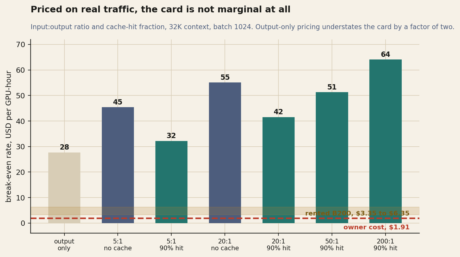
32K context, batch 1024, node time split between prefill and decode. Cache hits consume neither prefill nor decode, only a disk read.
Output-only pricing understates this card by roughly a factor of two. At a 20-to-1 input ratio with no caching, break-even is $55 per GPU-hour rather than $28.
At 200-to-1 with a 90 percent hit rate, which is what a long-running agent on a stable repository actually looks like, it is $64. Every one of those numbers is an order of magnitude above the rental market.
Cache hits are the mechanism. They consume no prefill and no decode, only a disk read of compressed entries plus a 5,504-token recompute, so raising the hit rate raises sustainable throughput without raising cost.
The $0.0028 price is low because the marginal cost is low, and it is worth having because it makes the traffic denser.
DeepSeek is not renting these GPUs
A rental rate contains a lessor’s margin, a scarcity premium that has been visibly volatile all year, and the lessor’s own financing cost. DeepSeek owns its fleet, and an owner’s cost is amortisation plus power.
Take a B200 at roughly $38,000 of capex, three years of life, 80 percent utilisation: $1.81 per GPU-hour. Add a kilowatt at PUE 1.3 and eight cents a kilowatt-hour: ten cents.
Call it $1.91 per GPU-hour all in, against a rental band of $3.35 to $6.35. An owner’s floor sits somewhere between 1.8 and 3.3 times below the price of renting the same silicon.
Note what power is and is not in that sum. A four-GPU node draws about 5.2 kW including overhead, which costs 42 cents an hour, which is under two percent of what the same node costs to rent. Power is not a meaningful line in the financial model.
It is a meaningful line in the physical one, and the report says so: the same paragraph that asks hardware vendors for a balance point also asks for more power headroom, because extreme kernel fusion drives compute, memory and network to high load simultaneously and power throttling becomes the limiter. Fusing everything is how you become thermally bound rather than bandwidth bound.
Which changes the verdict on the million-token window
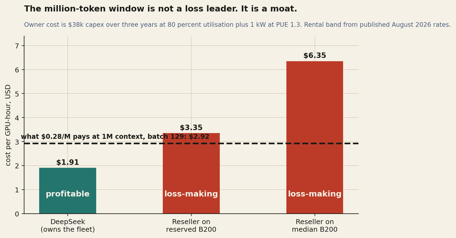
The break-even line is what $0.28 per million pays at 1M context with the batch capped at 129 by the KV pool.
Serving a million-token context at $0.28 per million output tokens needs a cost basis under $2.92 per GPU-hour. Nobody renting Blackwell has one. DeepSeek does, with room.
The million-token window is not a loss leader. It is a moat, and a precisely shaped one. Owner economics against rental economics
So the million-token window is not a loss leader. It is a moat, and a precisely shaped one. The twenty providers currently reselling the preview weights on OpenRouter at 37 percent below DeepSeek’s own card can do that at short context, where deep batches make the arithmetic work on rented hardware.
They structurally cannot do it at a million tokens, at that price, on rented Blackwell, because the KV pool caps the batch and the capped batch does not clear the rent. Which is presumably why none of them advertise it.
An open-weights MIT model whose most expensive capability is only economic for an owner-operator is a strange and rather elegant object. DeepSeek gave away the architecture, the mega-kernel and the kernel library, and kept the one thing that does not fit in a repository: a fleet, a request volume large enough to make the on-disk cache pay, and a cost basis a third of what anyone else can rent.
What the whole card is betting on
Put the three prices next to the three cost structures and the strategy is legible. Prefill is compute-bound and enormously profitable: at 35 percent MFU a node prefills roughly 485,000 tokens per second, which at $0.14 per million is $244 an hour against a node that costs $22 to rent and $8 to own. Decode is bandwidth-bound and needs deep batches.
Cache hits cost almost nothing and are priced almost at nothing, which makes them a throughput multiplier rather than a revenue line.
The card rewards exactly one traffic shape: high input-to-output ratio, high prefix reuse, deep concurrency, moderate context.
That is coding-agent and tool-calling traffic, which is what the 0731 post-training pass targeted, what the native Responses API and Codex adaptation are for, and what Quick Instruction and interleaved thinking were built to make cheaper. The architecture, the post-training, the serving stack and the price list are one artefact pointed at one workload.
Point a different workload at it, long single-turn document analysis with no prefix reuse and shallow concurrency, and the margin thins toward nothing even for DeepSeek. The card does not distinguish, yet. I do not expect that to last.
Reading the benchmarks in full
The report’s summary of its own results is accurate and selective, and the difference is worth spending a section on.
Start with the base models, which are the cleanest comparison in the document because all three ran in one internal harness with identical settings.
V4-Flash-Base carries 13B activated against V3.2-Base’s 37B, and 284B total against 671B. It should lose. It mostly does not.
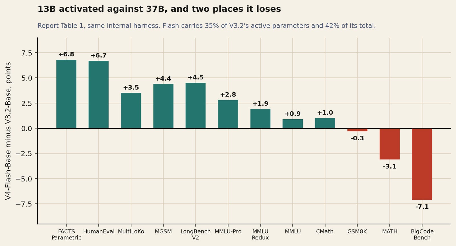
Report Table 1. Same harness, same settings. Flash carries 35 percent of V3.2’s activated parameters and 42 percent of its total.
Plus 6.8 on FACTS Parametric, plus 6.7 on HumanEval, plus 4.5 on LongBench-V2, plus 3.5 on MultiLoKo, plus 2.8 on MMLU-Pro.
Getting more world knowledge out of fewer total parameters is the surprising one, because knowledge retention is supposed to scale with parameter count and Flash has 42 percent of them.
And then two regressions that nobody discussing this model has mentioned. BigCodeBench falls 7.1 points, from 63.9 to 56.8. MATH falls 3.1, from 60.5 to 57.4. Those are not noise, they are the two largest deltas in the table after FACTS, and one of them is a coding benchmark on a model being marketed for coding agents.
Post-training clearly recovers a great deal of it, since the instructed model’s code-agent scores are strong. But the base model is worse at BigCodeBench than its predecessor and the report does not discuss why.
My guess, and it is a guess: BigCodeBench is a three-shot benchmark on library-heavy code, which is a knowledge task about API surfaces rather than a reasoning task, and it is the sort of long-tail recall that a smaller expert bank should hurt.
The world-knowledge gains going the other way argue against that, which is why it stays a guess.
Then the long-context claim. The report’s own summary says V4-Pro-Max delivers strong results with a one-million-token window, “surpassing even Gemini-3.1-Pro on academic benchmarks.” That is totally true.
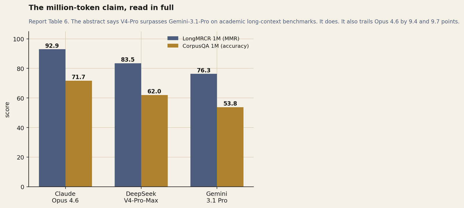
Report Table 6, DeepSeek’s own numbers, standardised configuration across models.
It is also the smaller half of the story. On LongMRCR at 1M, Claude Opus 4.6 scores 92.9, V4-Pro-Max 83.5, Gemini-3.1-Pro 76.3. On CorpusQA at 1M, Opus 71.7, V4-Pro-Max 62.0, Gemini 53.8. DeepSeek beats Gemini on both, comfortably, and loses to Opus by 9.4 and 9.7 points, in their own table, measured with their own harness.
Choosing Gemini as the comparison in the summary is a defensible framing decision and it is a framing decision.
The report is honest in other places where it did not have to be. It reports Terminal-Bench 2.0 at 67.9 on the original dataset while noting environment issues raised by another lab and disclosing that on the Verified subset V4-Pro scores about 72.0, which is higher.
It leaves cells blank for K2.6 and GLM-5.1 rather than filling them, saying those APIs were too busy to answer. It states that its reasoning performance trails the frontier by roughly three to six months.
That last sentence is in the report’s own summary of its own results and it is a more useful number than most third-party analysis of the same question.
What this does to everyone else’s floor
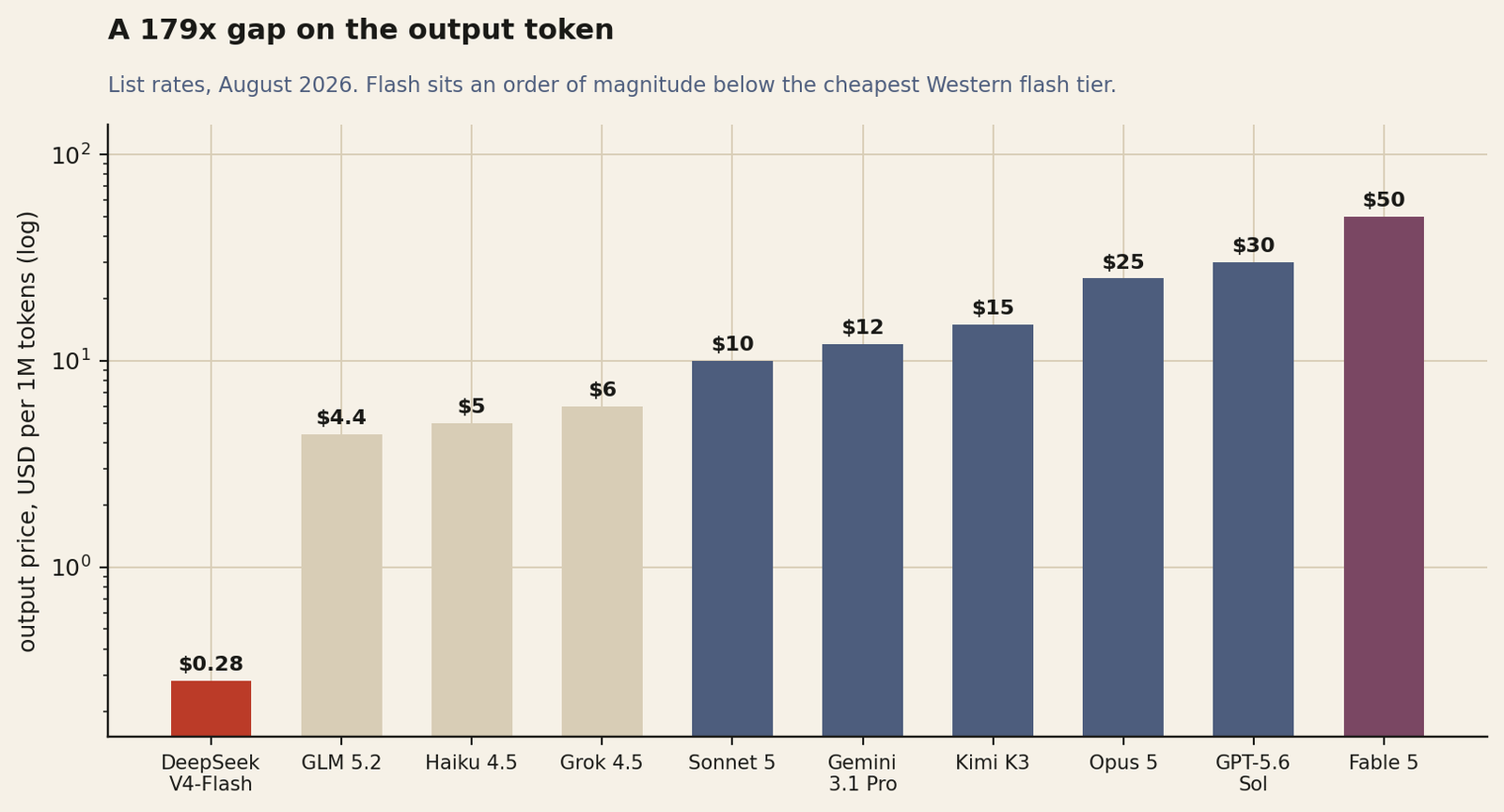
List rates, August 2026. The gap to the cheapest Western flagship is more than two orders of magnitude.
Reuters, reporting Artificial Analysis figures, put V4-Flash at roughly 3 cents to complete the Intelligence Index battery, against 86 cents for Kimi K3, $1.86 for GPT-5.6 Sol and $3.15 for Claude Fable 5.
On the index itself Flash scores 50, tying Gemini 3.6 Flash, one point behind GLM-5.2 and Muse Spark 1.1, seven behind Kimi K3, and nine or more behind Opus 5, Fable 5 and GPT-5.6.
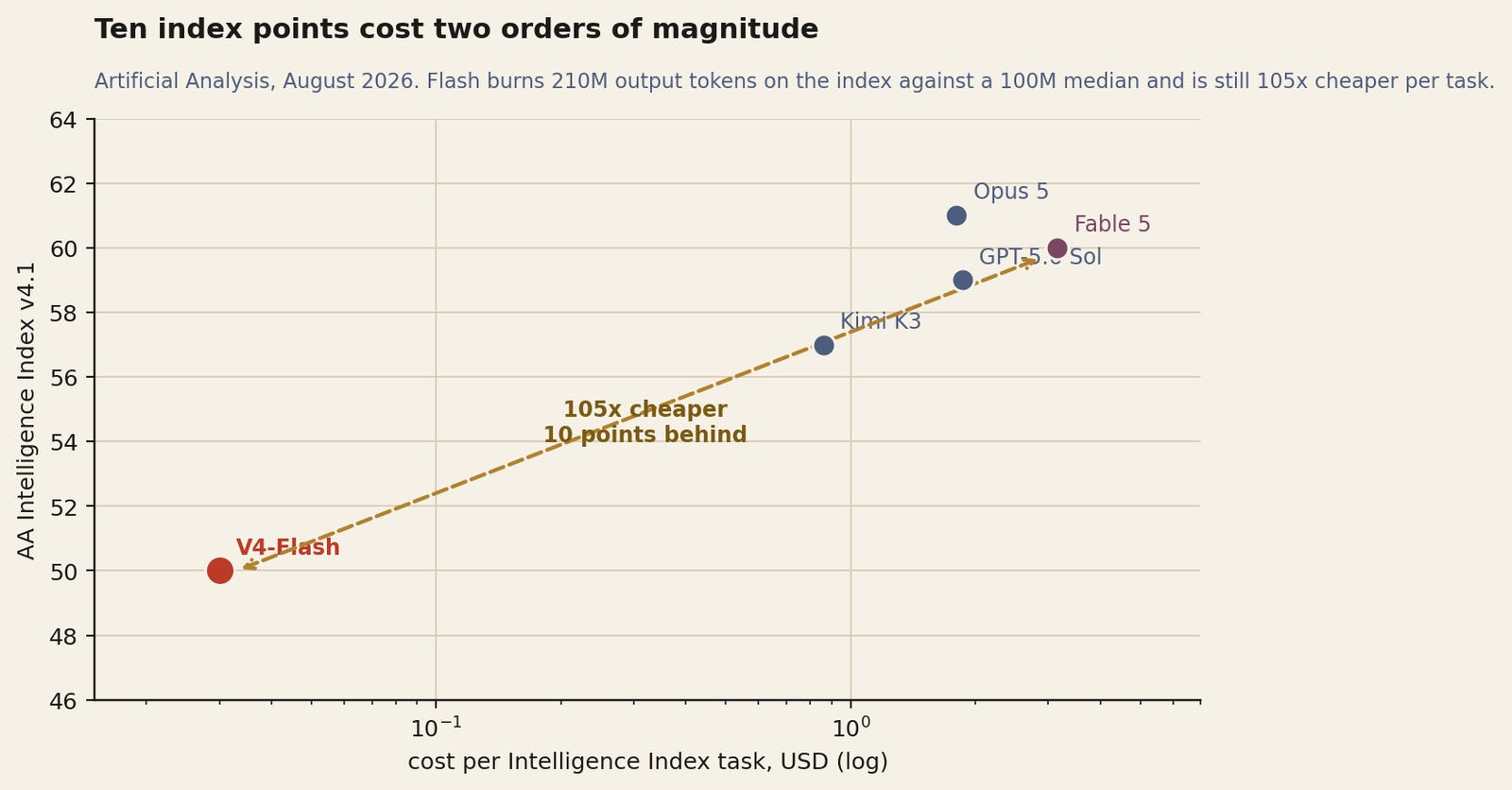
Artificial Analysis, August 2026. The vertical axis is nine points wide. The horizontal axis is two orders of magnitude.
The standard rebuttal to a cheap model is that it burns more tokens, so cost per task closes the gap that cost per token opens. It does not work here and the numbers say so precisely.
Flash generated 210M output tokens on the index against a 100M median, so it is 2.1 times more verbose than the typical model on identical work, for the documented reason that its Think Max system prompt instructs it to be. It is still 105 times cheaper per task than Fable 5, whose output token costs 179 times more.
Doubling token count against a 179x price advantage leaves 89x. The measured 105x is in that neighbourhood, and the verbosity tax is nowhere near large enough to matter.
What follows for the market is narrower than the headline suggests.
The nine-point index gap is not a rounding error. It is the difference between a model that finishes a hard task and one that plausibly fails it, and on hard agentic work a failed run costs more than the token price of a successful one.
At the top of the market price is not the binding constraint, and a 105x discount on a wrong answer is not a discount.
A 105x discount on a wrong answer is not a discount.On where the price pressure actually lands
The pressure is on the middle. Every workload running on a flagship because nobody bothered to route it, every classification and extraction and summarisation and first-draft call, is now paying somewhere between 60 and 105 times more than it needs to.
Routing is the mechanism that transfers that value and routing is engineering work most teams have not done. The models that should be nervous are not Opus 5 and Fable 5.
They are Haiku, Sonnet, the Flash and Terra and Luna tiers, everything between $1 and $5 per million output tokens where the capability gap to V4-Flash is small or negative and the price gap is 20x or more.
Two second-order effects are worth flagging. OpenRouter currently lists twenty providers serving the preview weights at $0.088 in and $0.176 out, 37 percent below DeepSeek’s own card.
That is an MIT-licensed model being resold below the price its author charges. Given the break-even analysis above, those hosts are running deeper batches, or cheaper capacity, or buying share. Only the first is durable.
And the weights are MIT, the mega-kernel is open inside DeepGEMM, the kernel library is open, and the fine-grained expert-parallel scheme was validated on Huawei Ascend as well as NVIDIA. The architecture is not the moat. The traffic shape is, and so is the on-disk cache that only pays off at DeepSeek’s request volume.
Where we might be wrong
The CSA and HCA layer split for Flash is inferred. The report says the first two layers are pure sliding window and the rest interleave, which for 41 remaining layers gives either 21 CSA and 20 HCA or the reverse.
We assumed the interleave opens with CSA. If it opens with HCA the cache figure moves from 3.372 to 3.216 GiB, about 5 percent, the parameter reconstruction moves by 13M, and nothing in the argument changes.
The B200 configuration is nameplate: 180 GB usable per GPU, 8 TB/s, four GPUs, 85 percent HBM utilisation, and a 63 percent achieved bandwidth fraction calibrated against a single third-party throughput measurement.
A production deployment with prefill and decode disaggregated across separate node pools has different and probably better economics than the single-pool model we used, and DeepSeek describes that disaggregation themselves.
The owner-cost figure of $1.91 per GPU-hour is built from a $38,000 capex assumption, a three-year life and 80 percent utilisation, none of which DeepSeek publishes. Capex at $30,000 gives $1.53 and at $45,000 gives $2.24, so the conclusion that an owner clears the 1M break-even survives the range, but only just at the top of it. The utilisation assumption is the fragile one: at 50 percent utilisation the figure is $2.99 and the verdict flips.
The blended-revenue model splits node time between prefill and decode on a single pool. Real serving disaggregates them across separate node pools with different shapes, which changes the split and generally improves it.
It also assumes cache hits consume no node time beyond the disk read, which understates their cost at high hit rates where storage bandwidth starts to bind.
The FLOPs reconstruction lands at 12.2 percent of V3.2 at 1M against the report’s 10 percent. The report measures in equivalent FP8 FLOPs while V4’s experts run FP4, which has identical peak throughput on current silicon but which the report says could be a third cheaper on future hardware.
That accounting difference is the likely source. My V3.2 indexer model may also be too generous.
The prefill MFU of 35 percent is an assumption, not a measurement, and both prefill revenue and the blended break-even scale linearly with it. At 20 percent the prefill figure drops from $244 an hour to $140 and every blended break-even in the traffic-mix chart falls by roughly a third.
Our reading of BigCodeBench’s regression as an API-recall effect is speculation and I have flagged it as such in the text. I would drop it entirely if the world-knowledge results did not cut the other way.
And the largest one. Every agent benchmark in the 0731 release is vendor-reported, measured with a harness DeepSeek has announced but not shipped, at maximum reasoning effort, with sampling parameters DeepSeek chose. Two of the nine suites are DeepSeek’s own internal sets. I have reproduced none of them and neither has anyone else.
Seven predictions, dated
By June 2027, at least one major Western lab ships a production model that compresses the KV cache along the sequence axis rather than the head axis. The mechanism is cheap, the memory win is fifty times, and it has now been demonstrated at 32T tokens of pre-training rather than in an ablation.
By 31 December 2026, someone publishes a sub-linear top-k selector for compressed attention, most likely hierarchical or learned-hash, and demonstrates it on V4’s open weights. The indexer being four fifths of attention cost at long context is too visible a target, and the FlashMemory work has already aimed at it from the prefetch side.
By March 2027, DeepSeek introduces context-length-tiered pricing, a peak-hour surcharge that actually activates, or both. A flat rate across a thirty times span of serving cost is not stable, and a surcharge has already been announced without being switched on.
By September 2027, at least one of Anthropic, OpenAI or Google cuts a mid-tier model’s output price by more than 50 percent without a corresponding capability release. The squeeze is on the middle of the ladder, not the top.
By the end of December 2027, DeepSeek-V5 or its equivalent replaces SwiGLU with a gate-free elementwise activation. The report asks for this explicitly in its hardware proposals, gives the reason (removing the gate projection lets the intermediate dimension grow under a fixed budget, which raises the interconnect balance point), and labs that publish that kind of request are usually describing work already underway.
By late June 2027, an SMT or ILP solver appears in the compilation pipeline of at least one other major inference stack. Z3 inside TileLang’s algebraic system is the first production instance I know of, the payoff is a few seconds of compile time for stronger vectorisation and bound analysis, and the idea travels.
By 31 December 2027, no model with a one-million-token context window is profitable at that context length on rented NVIDIA hardware at published rates, while remaining profitable for owner-operators. The KV pool caps concurrency, concurrency is what pays for decode, and the gap between owning and renting is wider than the margin. This is the prediction I expect to age worst, and it fails if HBM capacity per package jumps faster than I think.
Confidence dossier
Tier A · Stated in a primary source · 13 claims
43 layers, d=4096, m=4, m’=128, top-k 512, 256+1 experts, 6 activated
Report section 4.2.1, stated directlyPartial RoPE on exactly the last 64 dimensions; inverse RoPE at position -i on the output
Report section 2.3.3, stated directlyHCA has one KV stream and no indexer; CSA has two overlapping streams
Report equations 9 to 12 versus 20 to 23Attention sink logits per head, added to the softmax denominator
Report equation 27Hybrid Newton-Schulz, 8 steps at (3.4445, -4.7750, 2.0315) then 2 at (2, -1.5, 0.5)
Report section 2.4No QK-Clip, because RMSNorm on queries and KV entries already bounds the logits
Report section 2.4, stated as a deliberate omissionDense attention for the first 1T tokens; sparsity introduced at 64K with an indexer warmup
Report section 4.2.2Index scores quantised FP32 to BF16: 2x on top-k, 99.7 percent KV recall preserved
Report section 3.4Interconnect condition C/B <= 2 d_ff; 6144 FLOPs per byte for Pro
Report section 3.1, derived and evaluated thereThree on-disk SWA strategies; zero-caching needs n_win x L tokens of recompute
Report section 3.6.2Quick Instruction tokens reuse the existing KV cache to avoid a second prefill
Report section 5.1.1, Table 50731 is the same structure and size as the preview; post-training only
DeepSeek API changelog, 31 July 2026Rate card $0.14 / $0.0028 / $0.28 per million
Artificial Analysis and DeepSeek changelog, mutually consistent
Tier B · Derived here and cross-checked · 8 claims
Backbone reconstructs to 284.20B; MTP module excluded from the headline
Derived here from published constants, 0.07 percent residualAttention is 1.74 percent of weights and 39.3 percent of activated
Derived here; follows from the reconstructionmHC GEMM output dimension 24 = n_hc + n_hc squared + n_hc
Derived here; matches the figure quoted in report section 3.33.372 GiB of KV per 1M sequence at production precision
Derived here; four independent cross-checks, worst 10 percentIndexer is 79 percent of attention FLOPs at 1M, 50 percent at 32K
Derived here from published dimensionsAttention overtakes the expert bank at roughly 213K tokens
Derived here; sensitive to the CSA/HCA split assumptionFlash’s balance point is 4096 FLOPs per byte, 1.5x more demanding than Pro
Derived here by applying the report’s own condition to Flash’s d_ff5,504-token recompute restores the full SWA state, a 191x saving on prefill
Derived here from n_win, L and the activated parameter count
Tier C · Model output, assumptions named · 7 claims
129 concurrent 1M sessions on one 4xB200 node
Model; depends on 180 GB usable and 85 percent utilisation63 percent of peak HBM bandwidth achieved at low batch
Inferred from one third-party throughput measurement1M context clears at owner cost and not at any rental rate
Model output; hinges on the $38k / 3yr / 80 percent capex assumptionBlended break-even is 32 to 64 dollars per GPU-hour on agentic traffic mixes
Model output; single-pool prefill and decode, 35 percent prefill MFUOwner cost near $1.91 per GPU-hour against a $3.35 to $6.35 rental band
Model output; capex and utilisation assumed, power from published TDPBreak-even needs batch 256 at 32K against a $5.50 GPU-hour
Model output; single-pool assumption, no disaggregationPrefill grosses $244 an hour against a $22 node
Model output; 35 percent MFU is assumed, not measured
Tier D · Unreproduced or speculative · 3 claims
BigCodeBench regression is a long-tail API recall effect
Speculation, contradicted by the world-knowledge resultsAgent benchmark figures for the 0731 release
Vendor reported, unshipped harness, two internal suitesOpenRouter hosts undercutting DeepSeek by 37 percent are unprofitable
Speculative; their batch depth and capacity costs are unknown
Reproducing this
Everything numerical above comes from three short scripts with no dependencies beyond the standard library. None of it needs a GPU, because none of it is a measurement of a running model.
It is arithmetic over published constants, validated against figures published independently by vLLM and against ratios stated in the report itself.
The parameter reconstruction. Note the asymmetry between CSA and HCA in the projection count, which is the thing that is easy to get wrong:
L, d = 43, 4096
n_h, c, d_c = 64, 512, 1024          # query heads, head dim, query compression dim
n_hI, c_I   = 64, 128                # indexer heads, indexer head dim
g, d_g      = 8, 1024                # output projection groups
m, mp       = 4, 128                 # CSA and HCA compression rates
n_exp, n_sh, n_act, d_ff = 256, 1, 6, 2048
n_hc, V     = 4, 129280
n_swa, n_csa, n_hca = 2, 21, 20      # 2 SWA + 41 interleaved

per_expert = 3 * d * d_ff                        # SwiGLU: gate, up, down
moe_tot, moe_act = (n_exp+n_sh)*per_expert, (n_act+n_sh)*per_expert

def attn(kind):
    if   kind == ‘csa’: p = 4*d*c + 2*m*c        # two KV streams + positional biases
    elif kind == ‘hca’: p = 2*d*c + mp*c         # one KV stream  + positional bias
    else:               p = 1*d*c                # pure SWA, uncompressed
    p += d*d_c + d_c*(c*n_h)                     # query down then up
    if kind == ‘csa’:
        p += d_c*(c_I*n_hI) + d*n_hI             # indexer queries and per-head gate
    p += g*((n_h//g)*c)*d_g + (g*d_g)*d          # grouped output projection
    return p + n_h                               # attention sink logits

mhc = 2*(n_hc*d)*n_hc + (n_hc*d)*(n_hc**2)       # W_pre, W_post, W_res
att = n_swa*attn(’swa’) + n_csa*attn(’csa’) + n_hca*attn(’hca’)
backbone = L*moe_tot + att + 2*L*mhc + L*d*n_exp + 2*V*d
active   = L*moe_act + att + 2*L*mhc + L*d*n_exp

print(backbone/1e9, active/1e9)                  # 284.202  12.610
print(n_hc + n_hc**2 + n_hc)                     # 24, matching the mHC GEMM in section 3.3
The KV byte model, with all four calibration checks it has to pass before being used:
GiB, N = 1024**3, 1_048_576
c, c_I = 512, 128

def layer(kind, ent, idx, m=4, mp=128, n_win=128):
    if kind == ‘c4a’:   return (N//m)  * (ent + idx)
    if kind == ‘c128a’: return (N//mp) * ent
    if kind == ‘swa’:   return n_win * ent

# check 1: V3.2 bf16, MLA 512 latent + 64 rope, indexer 128, 61 layers
assert abs(61*(576*2 + 128*2)*N/GiB - 83.9) < 0.1              # vLLM publishes 83.9

# check 2: V4-Pro bf16, 30 c4a + 31 c128a, key and value shared
pro = 30*layer(’c4a’, c*2, c_I*2) + 31*layer(’c128a’, c*2, 0)
assert abs(pro/GiB - 9.62) < 0.01                              # vLLM publishes 9.62

# production precision: 64 rope dims bf16 + 448 fp8 = 576 B; fp4 indexer = 64 B
ent, idx = 64*2 + (c-64)*1, c_I//2
flash = 21*layer(’c4a’, ent, idx) + 20*layer(’c128a’, ent, 0) + 43*layer(’swa’, ent, 0)
v32   = 61*(64*2 + 512 + 128)*N

# check 3: the report’s own Figure 1 ratio
print(v32/flash)                       # 13.57  vs the report’s “13.7x smaller”

# check 4: the report’s claim that uncompressed SWA state is ~8x the compressed state
print(43*N*ent / (flash - 43*layer(’swa’, ent, 0)))            # 7.2  vs “approximately 8”

print(flash/GiB, flash/N)              # 3.372 GiB, 3453 bytes per context token
print(100*flash / (43*(2*8*128*2)*N))  # 1.96 percent of bf16 GQA-8, report says ~2
The decode roofline and break-even, for substituting your own hardware and rates:
NG, BW = 4, 8.0e12                                   # four B200, 8 TB/s each
w_step  = 278.1e9*0.5 + NG*6.2e9                     # FP4 experts + FP8 dense per rank
t_floor = w_step / (NG*BW)                           # 5.12 ms
eff     = t_floor / (1/122.7)                        # 0.63, from the measured 122.7 tok/s

def kv_bytes(ctx, ent=576, idx=64):
    return 21*((512+128)*ent + (ctx//4)*idx) + 20*(max(1, ctx//128)*ent + 128*ent)

def breakeven(batch, ctx, price=0.28):
    t = ((w_step + batch*kv_bytes(ctx)) / (NG*BW)) / eff
    return (batch/t) * 3600/1e6 * price / NG         # dollars per GPU-hour

print(breakeven(512, 32768))      # 14.76  clears the market comfortably
print(breakeven(256, 32768))      #  7.64  clears a mid-market B200
print(breakeven(129, 1048576))    #  2.93  clears nothing you can rent

# the report’s interconnect condition, applied to Flash
for name, d_ff in ((”Flash”, 2048), (”Pro”, 3072)):
print(name, 2*d_ff, “FLOP/Byte ->”, 4.5e15/(2*d_ff)/1e12, “TB/s at 4.5 PFLOP/s FP8”)Sources
DeepSeek-AI. DeepSeek-V4: Towards Highly Efficient Million-Token Context Intelligence. arXiv:2606.19348, 26 April 2026. Sections 2.2 to 2.4 for architecture, 3.1 for expert parallelism and the interconnect balance point, 3.2 for TileLang, 3.3 for batch invariance and determinism, 3.4 for FP4 QAT, 3.5 for the training framework, 3.6 for KV cache management and on-disk storage, 4.2 for the constants and the training schedule, 5.1 for post-training, 5.2 for RL infrastructure and DSec, 5.3 for evaluation.
vLLM Team. DeepSeek V4 in vLLM: Efficient Long-context Attention, 24 April 2026. Appendix contains the KV arithmetic used here for calibration, the derivation of why inverse RoPE is needed when key and value are shared, and the exact top-k values for c4a and c128a.
LMSYS. DeepSeek-V4 on Day 0: From Fast Inference to Verified RL with SGLang and Miles, 25 April 2026, for the MXFP8 by MXFP4 fused MoE path and the split-K mHC pre-GEMM kernel.
DeepSeek API changelog, 31 July 2026, for the 0731 release scope, the agent benchmark table and the harness settings.
Artificial Analysis, model page for DeepSeek V4 Flash 0731, accessed 5 August 2026, for Intelligence Index v4.1, output speed, time to first token, token volume and the rate card.
Reuters, via Quartz and Business Standard, 3 August 2026, for the cost-per-task comparison across V4-Flash, Kimi K3, GPT-5.6 Sol and Claude Fable 5.
Hugging Face model cards for deepseek-ai/DeepSeek-V4-Flash and deepseek-ai/DeepSeek-V4-Pro, for the mixed FP4 and FP8 weight format and the reference inference implementation.
DeepGEMM pull request 304, for the open-sourced MegaMoE fused expert-parallel kernel.
FlashMemory-DeepSeek-V4: Lightning Index Ultra-Long Context via Lookahead Sparse Attention, arXiv:2606.09079, for the Neural Memory Indexer follow-up and its own account of its limitations.
getdeploying.com B200 index (4 August 2026), gpuprice.fyi B200 index (31 July 2026) and published neocloud rate cards, for the $3.35 to $6.35 band.
Anthropic, OpenAI, Moonshot and Z.ai published rate cards as of 4 August 2026, for the price ladder.
Great post