
Decode Is Memory-Bound. Speculation Is the Arbitrage
Speculative decoding is the only inference optimization that turns idle silicon into tokens without changing a single output. Whether that lands on your bill as a discount or a surcharge is not a prop


Introduction
Rent a B200 for an hour and you are paying for roughly four and a half thousand trillion floating-point operations per second. Ask it to generate text from a seventy-billion-parameter model one user at a time, and for most of that hour the tensor cores do almost nothing.
The reason is not a bug, a bad kernel, or a scheduling failure. It is arithmetic. To produce a single token, the machine must read every weight in the model out of high-bandwidth memory, and reading is the slow part.
The multiply that follows the read is nearly free, and there is almost nothing to multiply, because a single decode step touches one token’s worth of activations against the entire weight matrix. You are paying for a fleet of trucks and using them to deliver one envelope per trip.
Put numbers on it. A seventy-billion-parameter model in the eight-bit precision typical of modern serving is seventy gigabytes of weights.
On a B200 with eight terabytes per second of memory bandwidth, sweeping those weights once takes just under nine milliseconds, and that single sweep yields exactly one token for one user.
The tensor cores that could have executed thousands of trillions of operations in that window execute a few billion. The arithmetic intensity of single-stream decode, the ratio of compute performed to bytes moved, sits at roughly one to two floating-point operations per byte.
The hardware does not break even until that ratio reaches several hundred. The gap between those two numbers is the entire subject of this issue, because that gap is compute you have already paid for and are not using.
Speculative decoding is the one technique in the inference toolbox that spends that idle compute on tokens, and, in its exact formulations, does so without altering the model’s output by a single logit. Every other lever trades something visible.
Quantization trades precision. Pruning trades capacity. Distillation trades a different model entirely. Speculation, done correctly, trades nothing the user can observe; it simply reorganizes when the weight reads happen so that one read can validate several tokens at once. That is what makes it unusual, and it is why every major laboratory shipped a version of it over the last eighteen months.
And yet the operator folklore says to turn it off above a certain batch size, and the operator folklore is correct, as far as it goes. The resolution of that apparent contradiction is the thesis of this piece.
The value of speculative decoding is not a number you can quote. It is a position on a plane whose axes are batch size and context length, measured against the ridge of the roofline. In one region it cuts your cost per token roughly in half.
In the adjacent region it raises your cost per token by a fifth. The technique never changed. The regime did. The job of this issue is to draw the plane, mark the line that divides it, and show why the workload that came to dominate 2026, long-form reasoning, walked straight into the half of the plane where speculation pays.
What speculation actually does, stated precisely
The mechanism is worth stating exactly, because almost every confusion about the economics traces back to a loose mental model of it.
A small, cheap model, the draft, proposes a short run of candidate tokens, say four or five of them, by generating them autoregressively in the ordinary way. Because the draft is small, those proposals are fast.
The large model, the target, then performs a single forward pass that scores all of the candidate positions at once. This is the move that matters: verifying four candidate tokens costs the target essentially one weight load, the same memory sweep it would have spent producing one token on its own, because the candidates are processed in parallel across the sequence dimension rather than one step at a time.
The target then walks the candidates left to right and applies a modified rejection-sampling test at each position.
It keeps the longest prefix of candidates that agrees with what it would have sampled itself, discards the first disagreement and everything after it, and emits one additional bonus token drawn from its own distribution at the point of divergence.
So a step that began with a draft of length K returns the number of accepted candidates, call it n, plus one. If the draft proposed five tokens and the target accepted three, the step produced four tokens for the price of one memory sweep. If the target accepted all five, it produced six. If it accepted none, it produced one, the bonus token, and you paid the draft’s cost for nothing.
This is the first thing the folklore gets right and the economics must respect: the speedup is governed by how many tokens the target accepts per step, and specifically by the accept length, the mean size of that accepted run plus the bonus.
It is not governed by the raw acceptance rate in isolation, and it is not governed by how clever the draft sounds. A draft that is right ninety percent of the time on the next token but falls apart by the third token buys you less than a draft that is right seventy percent of the time but stays coherent for five.
The lever is the length of the run, because each run, however long, costs exactly one expensive weight load of the target.
The lossleness property
For the rejection-sampling formulations introduced by Leviathan and colleagues in 2023 and independently by Chen and colleagues the same year, the output distribution is provably identical to standard autoregressive sampling from the target.
The modified rejection test is constructed precisely so that the accepted-token statistics match the target’s own. EAGLE preserves this exactly, as Hugging Face’s engineering writeup states plainly. The user cannot tell, from the output alone, that speculation was used.
That property deserves a caveat stated in the same breath, because vendors are not always careful about it. The losslessness holds for the exact rejection-sampling rule.
There are faster variants, relaxed acceptance, typical acceptance, and several aggressive tree-acceptance schemes, that raise the acceptance rate by loosening the test, and these do change the output distribution. They are often worth it.
But a quoted speedup that came from a relaxed acceptance rule is not the same artifact as a quoted speedup from exact rejection sampling, and an honest ledger keeps them in separate columns. When this issue later cites a four-times number, it will say which rule produced it.
The methods themselves form a clean lineage, and the direction of travel tells you what the field decided mattered. The original formulation used a separate draft model, a smaller member of the same family, which is simple but means maintaining and serving two models.
Medusa removed the second model by attaching several prediction heads to the target itself, each guessing a future position in parallel. EAGLE, in its first and second versions, moved the autoregression down a level, drafting in the target’s own feature space rather than in token space, which made the draft both cheaper and better aligned.
EAGLE-3, presented at NeurIPS 2025 and described in arXiv:2503.01840, pushed further: it fuses features from early, middle, and late layers of the target, predicts tokens directly rather than through an intermediate feature-regression step, removes a constraint that had limited how much training data helped, and uses a dynamic draft tree that expands the most promising candidates.
The endpoint of the lineage is to fold the draft into the target entirely, which is what DeepSeek’s multi-token prediction does, and which the next sections will show has economic consequences beyond mere convenience.
The roofline and the speculation budget
The previous issue, The Split and the Seam, derived the roofline for LLM serving in detail and split inference into its prefill and decode phases on exactly these grounds.
This issue assumes that derivation rather than repeating it, and reuses its house figures. The roofline says that for any kernel there is a ridge point, an arithmetic intensity above which you are limited by the chip’s compute throughput and below which you are limited by its memory bandwidth.
The ridge is simply peak compute divided by peak bandwidth. For an H100 SXM running FP8, that is one thousand nine hundred and seventy-nine teraFLOPS of dense tensor throughput against three and thirty-five hundredths terabytes per second of HBM3, which puts the ridge at five hundred and ninety-one FLOP per byte.
The H200 keeps the same compute but raises bandwidth to four and eight tenths terabytes per second, dropping the ridge to four hundred and twelve. A B200 at roughly four thousand five hundred teraFLOPS against eight terabytes per second sits near five hundred and sixty-two.
Single-stream decode operates at one to two FLOP per byte. Hold those two numbers next to each other. The operating point is two to nearly three orders of magnitude below the ridge.
That distance, expressed as a ratio, is the factor by which you could multiply the compute performed per byte moved before you would hit the memory ceiling and start paying for it in latency. Call it the speculation budget. On a single stream it is somewhere between three hundred and nearly six hundred times.
It is, very precisely, the ceiling on what any decode-side technique could reclaim from idle compute, and the headroom that speculative decoding draws on.

A reader should immediately ask why, if the budget is several hundred times, speculation delivers only two or three.
The answer is that no single technique spends the whole budget, and speculation in particular spends only a sliver of it.
Its yield is capped by accept length: each verification step still costs one weight load and returns at most the accepted run plus a bonus, which in practice is two to five tokens, so the multiple is bounded there no matter how much idle compute waits unused.
The draft is not free either, and its own forward passes consume part of the budget before any of it reaches the output. The rest of the headroom is what batching claims, the other and larger way to raise arithmetic intensity, and whatever neither mechanism reaches simply sits idle under the latency ceiling.
So the budget is the size of the prize, not the size of the winnings. Speculation is the instrument that collects the part of it that batching cannot, which, as the rest of this issue argues, is exactly the part that matters when a latency SLA forbids batching in the first place.
This budget is not an accident of one chip generation. It is the accumulated result of a divergence that has run for a decade.
Across the span from V100 to B200, tensor compute throughput grew by roughly thirty-six times, while HBM bandwidth over the same generations grew by only about nine times, a gap documented in the systems literature and discussed at length in this publication’s earlier piece on the memory wall.
Compute outran memory by a factor of four across those generations, and every factor of that divergence widened the speculation budget, because it pushed the ridge further above the place where decode actually runs.
The technique gets structurally more attractive with each generation of hardware that improves compute faster than bandwidth, which is to say, with each generation.
The budget is real, and finite
The roofline guarantees the headroom exists on a single stream. It does not guarantee the headroom survives batching, or long context. The next two sections are the story of what spends the budget down, and they reach opposite conclusions depending on which axis you move along.
The framing to carry forward is that speculation is, mechanically, a way of converting roofline headroom into tokens. When the headroom is large, the conversion is cheap and the tokens are nearly free.
When the headroom has been consumed by something else, there is nothing left to convert, and the draft’s compute becomes pure overhead.
Everything downstream is a question about how much headroom is actually available in your serving regime, and the surprising part, the part the folklore half-misses, is that the answer depends on two independent variables, not one.
Why batching is said to kill it
Here is the story every production guide tells, and it is the right place to start because it is true within its assumptions. As you raise the batch size, packing more concurrent sequences into each forward pass, the target’s arithmetic intensity rises.
The reason is that the weights are read once per step regardless of how many sequences are in the batch, so the cost of that read amortizes across the batch. One sequence pays the full one hundred and forty gigabyte sweep for one token.
Thirty-two sequences split the same sweep across thirty-two tokens. The bytes-per-token falls, the FLOP-per-byte rises, and at some batch size the target crosses its ridge and becomes compute-bound.
Past that crossing, the free headroom is gone, because the compute is now the scarce resource, and the draft model’s extra forward passes are competing for it against real work.
The crossing is commonly placed around a batch of thirty-two. Spheron’s production guide from March 2026 and E2E Networks’ engineering notes both put the practical break-even in that neighborhood, with the qualification that it moves with model size, quantization, and sequence length.
Below a draft acceptance of roughly one half, the guides agree, speculation hurts at any batch, because too few candidates survive verification to cover the draft’s cost.
The operational rule that falls out is blunt and widely repeated: disable speculation when batch sizes climb past the low tens, when outputs are short, when generation is high-entropy, or when you are memory-constrained on weights to the point that the draft displaces batch capacity.

The measured points anchor the shape. EAGLE 3.1, released jointly by the EAGLE, vLLM, and TorchSpec teams in May 2026 and benchmarked in the vLLM team’s own writeup running on Kimi-K2.6 in NVFP4 under vLLM with tensor parallelism of four on a GB200, delivered a per-user throughput multiple of two and three hundredths at concurrency one, one and seventy-one hundredths at concurrency four, and one and sixty-six hundredths at concurrency sixteen, on the SPEED-Bench suite.
The curve is unmistakable: the benefit is largest when the machine is emptiest, and it erodes as the batch fills. This is the empirical backbone of the folklore, and nothing in this issue disputes it on its own terms.
There is a sharper version of the same point that the practitioner Tian Pan has called the critical inversion. At low concurrency the draft runs in compute the target was wasting anyway, so it is free.
At high concurrency the draft’s forward passes contend with queued real requests for the same saturated compute, so the draft is no longer free; it is actively stealing throughput from work you could otherwise be doing.
Under that framing, speculation is fundamentally a low-concurrency latency optimization, and treating it as a throughput optimization at scale is a category error. This is good guidance. It is also, and this is the whole turn of the issue, an argument that silently assumes short context.
The amortization story is entirely about weights. It says the weight read, which dominates single-stream decode, gets cheaper per token as the batch grows. That is true. But the weight read is not the only thing decode reads from memory on every step, and the other thing it reads does not amortize across the batch at all.
The conventional wisdom is not wrong. It is two-thirds of a three-variable problem, and the missing variable is the one that 2026’s workloads turned up to eleven.
The KV cache re-opens the budget
Every token a transformer has already produced leaves behind a key and a value vector in every attention layer, and every future token must read all of them. That is the KV cache, and it is the second great memory cost of decode. Crucially, it behaves nothing like the weights.
The weights are shared across the batch, so their read amortizes. The KV cache is private to each sequence and grows with that sequence’s length, so its read scales with the batch size and with the context length simultaneously.
Doubling the batch does not split the KV read across more tokens; it doubles the total KV that must be read. Doubling the context length doubles it again.
The consequence is the result at the center of the MagicDec work, described in arXiv:2408.11049 and in Together AI’s analysis of it. There is a critical sequence length, call it S-star, beyond which the per-step KV read dominates the per-step weight read even at large batch.
Past S-star, decode is memory-bound again, not because the weights are unamortized, but because the KV cache is enormous and unamortizable. The free compute the conventional wisdom said batching had consumed comes back, because batching only consumed the part of the memory bill that the weights were responsible for. The KV part grew instead of shrinking.
This changes the geometry of the entire question. The compute-bound region is not the half-plane “batch greater than thirty-two.” It is a wedge: compute-bound requires high batch and short context, both at once. Move to small batch and you are memory-bound on weights. Move to long context and you are memory-bound on KV.
Only in the corner where the batch is large and the sequences are short does the target actually saturate its compute. Everywhere else, on a single stream, on long documents, on extended reasoning traces, the headroom is open and speculation has something to convert.
The short-context side of that corner has a hard edge worth naming. Because the KV cache caps how high arithmetic intensity can climb, there is a context length, roughly a thousand tokens on a B200 and closer to eleven hundred on an H200, past which no batch size reaches the compute-bound ridge at all.
That ceiling is the dashed wall in the diagram below, and the compute-bound wedge lives entirely to its left. Every reasoning trace sits far to its right.

Where the line actually sits
The boundary is not abstract; you can locate it with the model’s own dimensions, and where it lands is the punchline. Take a seventy-billion-parameter model of the Llama-3-70B shape: eighty layers, grouped-query attention with eight key-value heads of head-dimension one hundred and twenty-eight.
The key-value cache that must be read per token is two vectors, key and value, times eight heads, times one hundred and twenty-eight dimensions, times eighty layers, which is one hundred and sixty-three thousand eight hundred and forty elements per token.
In a sixteen-bit KV cache that is about three tenths of a megabyte for every token already in the sequence, per sequence. The weights, in an eight-bit serving format, are seventy gigabytes, read once per step and shared across the whole batch.
The crossover, the point where the per-step key-value read equals the per-step weight read, is therefore where batch size times sequence length reaches roughly seventy gigabytes divided by three tenths of a megabyte, which is about two hundred and twenty thousand.
That locus, batch times sequence held constant, is a hyperbola: it is the line drawn in Figure 3 below, and it marks where the KV read overtakes the weight read, which is to say where adding more batch stops reducing the bytes paid per token.
At a batch of thirty-two it puts that amortization crossover near seven thousand tokens; at a batch of sixty-four, near three thousand five hundred; at a batch of one hundred and twenty-eight, near one thousand seven hundred.
An eight-bit key-value cache roughly doubles all of those. This crossover is a finer fact than the compute-bound wall of the previous figure, and the two should not be confused: the wall is the context length past which no batch reaches the ridge, while the crossover is the point at a given batch where batching has stopped buying amortization.
The reasoning workload clears both at once. Hold it against the MLPerf numbers: a mean output of three thousand eight hundred and eighty tokens, a maximum of twenty thousand, AIME traces running to twenty-three thousand.
Those sequences run far past the roughly one-thousand-token compute-bound wall, so no batch reaches the ridge, and at any batch an operator can realistically run under a latency SLA they are past the amortization crossover as well. This is not a near miss.
The workload that came to define 2026 lives deep in the memory-bound region by a wide margin, which is the entire reason speculation pays there. (Both lines are house order-of-magnitude calculations from the stated architecture, graded in the dossier; the precise coefficients move with KV precision, head count, ridge, and serving format, but the order of magnitude, and therefore the conclusion, is robust.)

One honest qualification belongs here, because it is the first thing a careful reader will raise. The arithmetic above is for dense grouped-query attention, where the KV cache is large.
Architectures that compress the cache move the crossover to the right. DeepSeek’s Multi-head Latent Attention, by its hardware paper’s account, holds the KV cache to roughly seventy kilobytes per token, about a fifth of the dense-GQA figure, which pushes the crossover out toward a million aggregate tokens, the shallower line in the chart above.
DeepSeek-V4 goes further still: its model card reports that at a one-million-token context, V4-Pro spends about ten percent of V3.2’s KV cache and twenty-seven percent of its per-token compute, with V4-Flash at seven percent and ten percent, through a compressed sparse-attention stack.
This does not rescue the throughput regime. It relocates the line, and it does so precisely in service of making very long contexts affordable, which keeps sequences long, which keeps the budget open. The compression buys context length, and context length is what holds decode in the memory-bound region. The two facts point the same way.
MagicDec turns this into a working technique with one additional move: the draft itself must be light on KV, not just light on weights, or it reintroduces the very bottleneck it is trying to relieve.
With a draft that uses a fixed sparse or short-window KV footprint, MagicDec reports up to roughly two times on both throughput and latency together in the large-batch long-context regime on eight A100s, a regime where the conventional wisdom predicts speculation should be dead.
The reported draft-to-target memory ratio for a Llama-3.1-70B target with an eight-billion-parameter draft stays near four tenths and, importantly, stays constant as the batch grows, because the draft’s KV is bounded by design while the target’s KV grows.
That constancy is what keeps the draft cheap exactly where the conventional analysis assumed it would become expensive.
The corrected physics is therefore a single sentence with three clauses. Small batch is memory-bound because weights dominate. Long context is memory-bound because the KV read dominates.
Compute-bound is only the high-batch corner below the thousand-token wall, and that corner is smaller than the folklore implies. The “disable above batch thirty-two” rule is not wrong; it is a short-context rule wearing the costume of a general one.
And the moment your workload develops long sequences, whether from large documents or from long generations, the rule inverts, and speculation comes back to life precisely where you had been told to switch it off.
What actually shows on the ledger
Physics is not the bill. To get from the roofline to dollars, you have to know how the operator is allowed to set the batch size, and that is a question about service-level agreements, not about chips.
There are two serving regimes, and they read the same technique with opposite signs.
In throughput-maximizing service, the operator is free to batch all the way to the compute-bound point, because the only objective is cost per token and the way to minimize it is to amortize the weight read across as many sequences as possible. In that regime the machine is, by construction, saturated.
There is no idle compute. Speculation adds the draft’s forward passes to a chip that has nothing spare to run them in, so the cost per token rises. This is the regime the folklore is built for, and in it the folklore’s advice is exactly right.
In latency-capped service, the operator may not batch to the compute-bound point, because there is a ceiling on how long each token may take, and raising the batch raises per-token latency. The operator batches only until the latency SLA binds, and then stops, often well short of saturation.
The machine therefore runs with idle compute by design, not by accident, because the SLA forbids filling it. That idle compute is the speculation budget, and speculation converts it into tokens, cutting the cost per token. Same technique, opposite sign, and the only thing that changed was whether a latency ceiling capped the batch.
These two signs are not asserted; they fall out of a one-line cost model. Cost per token is the rental rate of the GPU divided by the tokens it delivers each second, so anything that multiplies throughput divides cost by the same factor.
In the latency-capped regime the wasted verification compute is free, because the chip sat idle under the SLA anyway, so throughput scales with the accept length discounted only by the draft’s own overhead: an accept length of about two and a half against a draft overhead near a fifth gives a throughput multiple close to two, which is the cut of roughly half the chart shows.
In the throughput-maximized regime the chip has no spare compute, so the draft’s wasted work bites directly. If the draft proposes three tokens and two and a half clear verification on average, the target spends three positions of compute to yield two and a half tokens, a throughput multiple near five sixths, which is the cost rise of about a fifth the chart shows.
The same two numbers, an accept length near two and a half and a draft length near three, generate both bars, and they are the same numbers behind the one-and-a-half to two-and-a-half times production speedups.
Push the draft length above the accept length and the throughput-regime penalty grows, which is precisely why over-drafting is the classic way to lose money on speculation in a saturated cluster.

The reason latency-capped service is the common case in 2026, rather than a corner case, is written directly into the benchmark SLAs.
MLPerf Inference v5.1, published by MLCommons in September 2025, sets for its DeepSeek-R1 reasoning workload a time-to-first-token ninety-ninth-percentile threshold of two seconds and a time-per-output-token ninety-ninth-percentile threshold of eighty milliseconds, against a mean input of around eight hundred tokens and a mean output of three thousand eight hundred and eighty, with a maximum output of twenty thousand, the highest the benchmark has ever specified.
An eighty-millisecond ceiling on per-token latency, applied to sequences thousands of tokens long, caps the batch far below the compute-bound point, because long sequences mean large KV reads and large KV reads mean each added unit of batch costs latency you do not have.
The SLA traps the GPU in the memory-bound regime. The trap is the opportunity: a memory-bound GPU has idle compute, and idle compute is what speculation eats.
The benchmark concedes the point
The argument stops being a thesis and becomes a rule when the benchmark authority writes it into the rules. In March 2026, MLPerf Inference v6.0 added an interactive reasoning scenario for DeepSeek-R1 with the ceiling pulled tighter still, a 1.5-second TTFT and a 15-millisecond TPOT at the ninety-ninth percentile.
To make that scenario achievable at all, MLCommons mandates speculative decoding for it: implementations must run the official DeepSeek-R1 MTP head with EAGLE-style decoding.
The independent body that defines how inference is measured decided that, past a certain latency target on reasoning traffic, speculation is not an optional optimization but a requirement of entry.
The dollar figures that frame the chart are anchored to 2026 market rates and published per-token costs, kept deliberately conservative. Neocloud H100 capacity runs around two dollars an hour, with Spheron listing two dollars and one cent; B200 on-demand sits in the five-to-six-dollar range across getdeploying and aimultiple’s trackers.
Published serving costs land near forty-two cents per million tokens on a B200 and forty-seven cents on an H100 PCIe. The point of the chart is not to nail a single deployment’s economics to the cent, which would be dishonest given how much rate, model, and quantization move the number.
The point is the asymmetry: the same forty-something cents per million can become a discount or a surcharge depending solely on which side of the saturation line your SLA puts you.
The most honest evidence for this whole framing comes, unexpectedly, from the vendor with the most incentive to claim an unqualified win. DeepSeek’s hardware paper, arXiv:2505.09343, states that its multi-token prediction module can slightly hurt raw throughput while significantly improving end-to-end generation latency.
Read that again in the context of the two regimes. DeepSeek is reporting, in print, that in a throughput accounting MTP can cost a little, and in a latency accounting it helps a lot, and that they ship it because latency is the product.
They add a second-order point that sharpens it further: MTP raises the effective batch size, which in their mixture-of-experts architecture increases expert-parallel arithmetic intensity, partially offsetting the throughput cost.
A company could have quoted the latency win alone and called it a free lunch. Instead they documented the tradeoff in both directions, which is precisely the shape of the real ledger this issue is arguing for.
When the vendor with the strongest incentive to claim a pure throughput win instead publishes that the technique “slightly hurts throughput while significantly improving latency,” that is not a weakness in the technique.
It is the ledger showing its true two-sided shape, in the vendor’s own numbers.
Why reasoning moved the bill into decode
Cost per token has a denominator, and the denominator is dominated by decode steps, because prefill is a single parallel pass over the prompt while decode is a long sequence of memory-bound steps, one per output token.
Anything that multiplies the number of output tokens multiplies the share of the bill that lives in decode, which is exactly the share speculation can attack. This is why 2026 is a different economic environment for speculative decoding than 2023 was, even though the technique is largely the same. The traffic changed.
Reasoning models emit output on a different scale entirely. A conventional chat reply is a few hundred tokens. A reasoning trace runs to thousands, and the trend within the model generation has been sharply upward: BentoML’s deployment guide notes that DeepSeek-R1-0528 nearly doubled its reasoning length over the prior R1, from around twelve thousand to around twenty-three thousand tokens on a single hard math question.
MLPerf’s DeepSeek-R1 workload puts the mean output at three thousand eight hundred and eighty and the maximum at twenty thousand. Agentic systems then chain many such traces into a single user-visible task, so the effective output length per task can be larger still.
The bill, which used to be split between a substantial prefill and a modest decode, has tilted hard toward decode.

Two facts about reasoning traffic place it squarely in the regime where speculation pays. The first is the one just shown: it is decode-heavy, so the part of the bill speculation can lower is the dominant part. The second is subtler and follows from the previous sections.
Long traces mean long sequences in flight, which means large KV reads, which means decode is memory-bound even when the operator manages to batch, both because the latency SLA caps the batch and because the KV cost re-opens the budget past S-star.
The two mechanisms reinforce each other. The workload is in the memory-bound regime by virtue of its output length, and it is held there by virtue of its latency SLA. There is idle compute on the machine for both reasons at once, and speculation is the technique that turns idle compute into tokens.
The architectural direction of travel keeps the budget open rather than closing it. DeepSeek-V4’s sparse-attention work, with V4-Pro reportedly using about twenty-seven percent of the FLOPs and ten percent of the KV of V3.2 at a one-million-token context through DeepSeek Sparse Attention, is explicitly aimed at making very long contexts affordable.
Cheaper long context means more long context, which means more memory-bound decode, which means a wider speculation budget, not a narrower one. The hardware trend widens the budget by improving compute faster than bandwidth; the model trend widens it by pushing context length up. Both vectors point the same way.
And this is where accept length, the lever from the first section, cashes in directly against the denominator. The decode discount is, to first order, the accept length: a method that lands two and a half accepted tokens per step is doing roughly two and a half times the decode work per expensive weight load.
The measured accept lengths of the shipped 2026 methods, two and fifty-five hundredths for DeepSeek-V3.2’s MTP, two and seventy-six hundredths for GLM-5’s shared-MTP design, and four and seven tenths for EAGLE-3 on coding and reasoning workloads, are therefore not abstract quality scores.
They are multipliers on the largest line item in the reasoning-era bill.

Where speculation loses
A technique that only ever helps does not need an issue written about when to use it. Speculation has real failure modes, and an analysis that buries them is worth less than one that lists them, so here is the full debit column, without hedging.
The throughput regime. In saturated high-batch short-context serving, the offline-batch corner of the phase diagram, speculation is a tax and should be disabled. The compute is fully employed, the draft has nothing free to run in, and its forward passes displace real work. The Spheron and Tian Pan guidance is correct here without qualification. If your job is to push the maximum number of short completions through a fleet of GPUs at minimum cost per token, speculation is the wrong lever.
Acceptance collapse. Below roughly one-half acceptance, speculation hurts at any batch, because too few candidates survive to cover the draft’s cost. Acceptance is not a constant; it falls with high sampling temperature, with out-of-distribution inputs the draft was never trained on, and with the kind of high-entropy generation where the next token is genuinely uncertain. A draft trained against one target distribution and then serving a drifted or fine-tuned target degrades silently, the acceptance rate sliding without any error being raised. Monitoring accept length in production is not optional; it is the only way to notice that your discount has quietly become a surcharge.
VRAM pressure. The draft model and its KV cache occupy memory you could otherwise spend on a larger batch or a longer context. A Llama-3.3-70B target in FP8 alongside a one-billion-parameter draft consumes roughly seventy-five to seventy-eight gigabytes on an eighty-gigabyte H100, per Spheron’s figures, leaving very little headroom. On a memory-constrained deployment, the draft can cost you more in lost batch capacity than it returns in accept length, and that tradeoff has to be measured, not assumed.
No help for time-to-first-token. Speculation accelerates decode, and only decode. It does nothing for prefill, which means it does nothing for time-to-first-token. Under the MLPerf two-second TTFT ceiling, that is a separate problem requiring separate techniques, which is precisely the prefill-decode disaggregation argument of Issue 03. Speculation and prefill optimization are complementary, not substitutes, and a serving stack that needs both will not get the first from the second.
Draft maintenance. A separate draft model is a second training, evaluation, and deployment surface that must be kept aligned as the target evolves. Every target update risks degrading a draft that was tuned against the previous version. EAGLE-style heads and built-in MTP layers reduce this by coupling the draft to the target’s own features or parameters, but they do not eliminate the obligation to retrain and revalidate. GLM-5’s choice to share parameters across three MTP layers, described in arXiv:2602.15763, is partly an answer to exactly this maintenance cost: fewer independent parameters to train and keep aligned.
The losslessness caveat, restated. The provable equivalence to standard sampling holds for the exact rejection-sampling rule. Relaxed acceptance, typical acceptance, and aggressive tree-acceptance schemes raise throughput by changing the output distribution. They are frequently worth it, but a four-times figure obtained under a relaxed rule is not interchangeable with a four-times figure under exact sampling, and a serving team quoting a speedup owes itself, and its users, clarity about which rule produced it.
Draft-length tuning. The number of tokens the draft proposes per step, often written gamma, is a workload-dependent knob with a real optimum. Set it too long and the draft burns compute generating candidates that will be rejected; set it too short and you leave accept length on the table. The optimum moves with acceptance rate and with batch size, so a value tuned on one workload can be wrong on another, and dynamic schemes that adjust it per request exist precisely because no single value is right everywhere.
The lab-versus-production gap. The EAGLE-3 paper reports speedups of up to six and a half times, but those are temperature-zero academic measurements on Vicuna-13B, Llama-3.1-8B, and Llama-3.3-70B. Production reports cluster instead around two to three times: LMSYS and Vertex describe two-to-three-times figures for EAGLE-3 on SGLang, E2E Networks reports two and three tenths on Llama-3.1-8B at a batch of four, and a Gemma-4 EAGLE3 draft head is documented at one and seventy-two hundredths at batch one on conversational traffic. The gap between the lab number and the production number is itself one of the most important facts in this space, because quoting the former as if it were the latter is the single most common honesty failure in vendor material on speculative decoding.

A decision on the plane
The verdict is not a yes or a no. It is a lookup. Given a workload’s batch size, its context length, its latency SLA, and its measured acceptance, the phase diagram tells you which regime you are in, and the regime tells you the sign of the ledger. The table below collapses the analysis into that lookup.
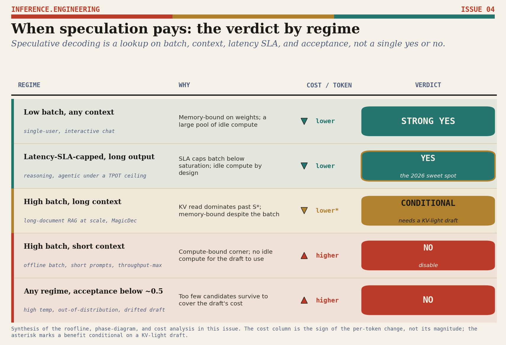
State the thesis cleanly now that the machinery is in place. Speculative decoding is the only inference technique that converts decode’s idle compute into tokens losslessly, and the sign of its effect on your bill is set entirely by whether that compute was actually idle.
Whether it was idle is a question about the roofline, and where you sit on the roofline is a question about batch size and context length, the two axes of the phase diagram.
There is no universal answer because the inputs are not universal. There is a correct answer for every point on the plane, and the table is how you read it.
The reason this matters more now than it did three years ago is that the median workload moved. In 2023 the prototypical request was a short chat completion at modest context, which lives near the compute-bound corner once you batch it, where speculation is at best neutral.
In 2026 the prototypical high-value request is a long reasoning trace under a tight per-token latency SLA, which lives deep in the memory-bound region for two independent reasons, its output length and its SLA, and which is therefore exactly where speculation pays. The technique did not move toward the workload. The workload moved toward the technique.
That migration is why the shipping decisions of the major laboratories converged. DeepSeek built multi-token prediction into V3 and carried it through V3.2, documenting the latency win and the throughput cost honestly.
GLM-5 shipped a shared-parameter three-layer MTP design with a measured accept length near two and three-quarters. NVIDIA’s NeMo RL work applied EAGLE-3 to reinforcement-learning rollouts and reported a one-and-eight-tenths-times generation speedup at the eight-billion scale, with validation accuracy on AIME-2024 evolving identically under autoregressive and speculative decoding, a clean confirmation that the lossless guarantee holds across training.
EAGLE-3 landed across vLLM, SGLang, and TensorRT-LLM, the three serving stacks that matter. These are not independent fashions. They are the same bet, placed by everyone who looked at the same plane and saw that reasoning traffic had walked into the half where the ledger reads in your favor.
The technique never changed. The regime did. Speculation lowers your cost per token exactly where batching cannot help you, and reasoning is the workload that made that region the center of the map.
Confidence tiers and external-audit read
Every load-bearing claim in this issue is scored below against a four-tier confidence scale, with its source named inline.
The scale is applied as an external auditor would apply it, crediting primary and measured sources, discounting derived and illustrative ones, and flagging the weakest links explicitly rather than hiding them in the prose.
Tier A primary or measured: peer-reviewed papers, vendor hardware disclosures, MLPerf-published SLAs and benchmark statistics.
Tier B secondary, with method: vendor or practitioner reports that state their configuration and measurement conditions.
Tier C derived or stylized: house figures and curves built from the cited physics, presented as illustrative renderings, not measurements.
Tier D illustrative or round-number: reference values chosen for scale, not claimed as measured.
A
Exact rejection-sampling speculative decoding is output-distribution lossless.
Leviathan et al. 2023; Chen et al. 2023; EAGLE losslessness per Hugging Face engineering writeup. Provable equivalence to standard sampling under the exact rule.
A
EAGLE-3 mechanism: training-time test, multi-layer feature fusion, direct token prediction, dynamic draft tree.
EAGLE-3 paper, NeurIPS 2025, arXiv:2503.01840. Headline lab speedups up to 6.5x at temperature 0 on Vicuna-13B, Llama-3.1-8B, Llama-3.3-70B (explicitly a best-case lab figure; production lands far lower, see Figure 8).
A
DeepSeek MTP slightly hurts throughput while significantly improving end-to-end latency; raises effective batch and expert-parallel intensity.
DeepSeek hardware paper, arXiv:2505.09343. The two-sided tradeoff is stated in the vendor’s own text, which is the strongest single piece of evidence in this issue.
A
MLPerf DeepSeek-R1 SLAs: TTFT 99p 2s, TPOT 99p 80ms; mean input 800, mean output 3,880, max output 20,000.
MLPerf Inference v5.1, MLCommons, September 2025. These SLAs are the anchor for why latency-capped serving traps the GPU in the memory-bound regime.
A
MLPerf Inference v6.0 added a DeepSeek-R1 interactive scenario (TTFT 1.5s, TPOT 15ms) and mandates speculative decoding (official MTP head, EAGLE-style) to meet it.
MLCommons, March 2026. The benchmark authority requiring speculation for tight-latency reasoning is the strongest external corroboration of the thesis.
A
NVIDIA NeMo RL: EAGLE-3 gives ~1.8x rollout generation speedup at 8B; AIME-2024 accuracy identical under autoregressive and speculative decoding throughout training.
NVIDIA NeMo RL research, May 2026. Independent empirical confirmation that the lossless guarantee holds in practice across training.
A
Critical-sequence-length result: past S*, decode is memory-bound even at large batch via KV read; KV-light draft delivers up to ~2x throughput and latency.
MagicDec, arXiv:2408.11049; Together AI long-context analysis. Draft-to-target memory ratio ~0.4, constant at large batch, for Llama-3.1-70B with 8B draft.
A
Roofline ridge points: H100 SXM FP8 591, H200 412, B200 ~562 FLOP/byte; compute outgrew bandwidth ~36x vs ~9x V100 to B200.
Carried from Issue 03, The Split and the Seam, and Issue on the memory wall, The Wall and the Stack. Hardware specifications and systems-literature divergence figures.
A
DeepSeek-V4 sparse attention: V4-Pro 27% FLOPs and 10% KV of V3.2 at 1M context; V4-Flash 10% and 7%.
Official DeepSeek-V4-Pro / V4-Flash model cards (Compressed Sparse Attention + Heavily Compressed Attention). Verified figures. Direction-of-travel evidence that long context is getting cheaper, widening the budget.
A
EAGLE 3.1 per-user throughput: 2.03x at concurrency 1, 1.71x at 4, 1.66x at 16.
Primary: vLLM team blog, May 2026 (EAGLE / vLLM / TorchSpec joint release). Kimi-K2.6-NVFP4, tensor-parallel 4, GB200, non-disagg, SPEED-Bench coding. Verified against the primary engineering writeup.
B
Practical break-even near batch 32; below ~0.5 acceptance speculation hurts at any batch.
Spheron production guide, March 2026; E2E Networks. Practitioner guidance with stated qualifications on model, quantization, and sequence length.
B
The lab-versus-production speedup comparison in Figure 8 (6.5x lab vs a 1.66 to 2.3x production cluster).
Compiled from verified primary and vendor sources (EAGLE-3 paper, EAGLE 3.1 vLLM blog, DeepSeek hardware paper, Gemma-4 EAGLE3 card, E2E Networks). Bars use different targets and conditions and are not strictly comparable; shown to convey range, not to rank.
B
Production speedups cluster at 2 to 3x; E2E reports 2.3x on Llama-3.1-8B at batch 4, accept length 4.5 to 5.0.
LMSYS and Vertex on SGLang; E2E Networks. Multiple independent practitioner reports converging on the same range.
B
Accept lengths: DeepSeek-V3.2 MTP 2.55, GLM-5 shared-MTP 2.76; GLM-5 shares parameters across 3 MTP layers.
GLM-5 technical report, arXiv:2602.15763. EAGLE-3 accept length 4.5 to 5.0 from E2E Networks.
B
2026 GPU rates and per-token costs: H100 ~$2/hr, B200 ~$5 to $6/hr on-demand; ~$0.42/M (B200), ~$0.47/M (H100 PCIe).
Spheron ($2.01/hr H100), getdeploying, aimultiple. Market trackers; rates move with provider, commitment, and region.
B
Reasoning length growth: R1-0528 nearly doubled to ~23K tokens per AIME question vs ~12K for prior R1.
BentoML DeepSeek deployment guide, 2026. R1 token pricing ~$0.55/M in, ~$2.19/M out; output billed higher and dominates cost.
C
The KV-versus-weight amortization crossover (Figure 4): batch x sequence near 220,000 for a 70B model, where the KV read overtakes the weight read (~7,000 tokens at batch 32, ~1,750 at batch 128).
House order-of-magnitude calculation from Llama-3-70B architecture (80 layers, 8 KV heads, head-dim 128) and the weight-versus-KV read balance, drawn in Figure 4. The coefficient moves with KV precision and serving format; the order of magnitude, and the conclusion that reasoning traces sit past the crossover, is robust.
C
The compute-bound boundary and ~1,000-token wall in Figure 3.
Derived, not stylized: the boundary is the roofline condition AI = 2B/(1+B*S/C) exceeding the ridge, with the wall at S = 2C/R (C ~ 220,000; R = 562 FP8 for B200). A house calculation with standard simplifying assumptions (GEMM-dominated FLOPs, dense GQA KV); exact coordinates shift with precision and ridge, the structure does not.
C
The -48% / +19% cost magnitudes in Figure 5.
Derived from the cost model in the text (accept length ~2.5, draft length ~3, draft overhead ~0.2) and consistent with the production speedups in Figure 8. Absolute dollar levels still vary with rate, model, and quantization; the regime-dependent sign and rough magnitude are the load-bearing claim.
C
The shape of the speedup-decay envelope in Figure 2.
House curve illustrating the conventional decay toward break-even; the measured EAGLE 3.1 points on it are Tier A and the break-even location is sourced, but the connecting envelope is schematic, not fitted.
D
The ~300-token chat-reply baseline and the vanilla-draft 2.1 accept-length reference.
Round-number references chosen to set scale against the measured reasoning and method figures, not claimed as measured values.
External-audit simulation
Audited as a whole, the issue rests on a spine of Tier A primary sources, and every load-bearing empirical claim in it was checked against its primary source: the EAGLE-3 paper (arXiv:2503.01840), MagicDec (arXiv:2408.11049), the DeepSeek hardware disclosure (arXiv:2505.09343), the GLM-5 report (arXiv:2602.15763), the MLPerf v5.1 and v6.0 specifications, the DeepSeek-V4 model cards, and the EAGLE 3.1 vLLM release each confirmed the figures attributed to them.
The central argument, that the sign of the ledger is set by serving regime and that reasoning traffic sits in the favorable regime, follows from those sources rather than from the house figures, which is the property an audit most wants to see.
Two pieces of evidence are doing disproportionate work and both survive scrutiny: DeepSeek’s own statement that MTP slightly hurts throughput while significantly improving latency, a direct vendor quote, and MLPerf v6.0’s decision to mandate speculative decoding for its tight-latency reasoning scenario, which is the measuring authority writing the thesis into the rules.
The weakest links are named rather than hidden, and after this revision they are narrow. Boundary and Crossover are now derivations rather than stylizations: the first is the roofline condition with the wall at twice the bytes-ratio over the ridge, the second is the weight-versus-KV balance, both house calculations carried out with standard simplifying assumptions (GEMM-dominated compute, dense grouped-query KV) whose exact coordinates move with precision and ridge while the structure holds.
The cost magnitudes are likewise derived from an explicit model, an accept length near two and a half and a draft length near three, and cross-checked against the production speedups; what remains genuinely soft there is the absolute dollar level, which varies too much with rate, model, and quantization to pin down.
The decay envelope is a schematic shape, though the measured points on it and its break-even location are sourced. The chat and vanilla-draft baselines are round numbers for scale. A handful of practitioner figures, the break-even batch, the VRAM envelope, and the production speedup band, come from individual engineering guides rather than independently reproduced benchmarks, and are tiered B accordingly.
None of these elements carries the conclusion: a reader who accepts only the Tier A claims, and works the two house calculations independently, arrives at the same verdict table.
Overall confidence in the thesis is high, because the thesis is a statement about regimes and signs that the primary sources support directly, and it is deliberately not a statement that speculation yields any specific universal multiple, which the evidence would not support.
The quantitative illustrations are held at lower confidence by design, and labeled as such, so that the argument does not borrow credibility it has not earned. A reader who accepts only the Tier A claims still arrives at the same verdict table; the lower tiers furnish the texture, not the conclusion.
Sources and useful informations
Primary and secondary sources for the load-bearing claims, with arXiv identifiers and venues where applicable. The text above attributes each source at its point of use; this is the consolidated record.
Papers appear first, then benchmark specifications, vendor and practitioner writeups, and model cards.
Y. Leviathan, M. Kalman, and Y. Matias. Fast Inference from Transformers via Speculative Decoding. International Conference on Machine Learning (ICML), 2023. arXiv:2211.17192.
C. Chen, S. Borgeaud, G. Irving, J.-B. Lespiau, L. Sifre, and J. Jumper. Accelerating Large Language Model Decoding with Speculative Sampling. arXiv:2302.01318, 2023.
T. Cai, Y. Li, Z. Geng, H. Peng, J. D. Lee, D. Chen, and T. Dao. Medusa: Simple LLM Inference Acceleration Framework with Multiple Decoding Heads. International Conference on Machine Learning (ICML), 2024. arXiv:2401.10774.
Y. Li, F. Wei, C. Zhang, and H. Zhang. EAGLE: Speculative Sampling Requires Rethinking Feature Uncertainty. International Conference on Machine Learning (ICML), 2024. arXiv:2401.15077.
Y. Li, F. Wei, C. Zhang, and H. Zhang. EAGLE-2: Faster Inference of Language Models with Dynamic Draft Trees. Conference on Empirical Methods in Natural Language Processing (EMNLP), 2024. arXiv:2406.16858.
Y. Li, F. Wei, C. Zhang, and H. Zhang. EAGLE-3: Scaling up Inference Acceleration of Large Language Models via Training-Time Test. Conference on Neural Information Processing Systems (NeurIPS), 2025. arXiv:2503.01840.
R. Sadhukhan, J. Chen, Z. Chen, V. Tiwari, A. May, T. Chen, and B. Chen. MagicDec: Breaking the Latency-Throughput Tradeoff for Long Context Generation with Speculative Decoding. arXiv:2408.11049, 2024.
DeepSeek-AI. DeepSeek-V3 Technical Report. arXiv:2412.19437, 2024.
DeepSeek-AI. Insights into DeepSeek-V3: Scaling Challenges and Reflections on Hardware for AI Architectures. International Symposium on Computer Architecture (ISCA), 2025. arXiv:2505.09343.
DeepSeek-AI. DeepSeek-R1: Incentivizing Reasoning Capability in LLMs via Reinforcement Learning. arXiv:2501.12948, 2025.
Z.ai (Zhipu AI). GLM-5 Technical Report. arXiv:2602.15763, 2026.
MLCommons. MLPerf Inference: Datacenter, v5.1 (DeepSeek-R1 reasoning workload). Benchmark rules and results, 2025.
MLCommons. MLPerf Inference: Datacenter, v6.0 (DeepSeek-R1 Interactive scenario, mandated speculative decoding). Benchmark rules, 2026.
EAGLE Team, vLLM Team, and TorchSpec. EAGLE 3.1: release and SPEED-Bench results on Kimi-K2.6. vLLM Blog, May 2026.
NVIDIA. Speculative Decoding for Reinforcement-Learning Rollouts in NeMo RL. NVIDIA Developer technical writeup, 2026.
Together AI. Speculative decoding for high-throughput long-context inference (analysis of MagicDec). Together AI Blog, 2024.
BentoML. The Complete Guide to DeepSeek Models: V3, R1, V4 and Beyond. BentoML Blog, 2026.
Spheron Network. Speculative decoding in production: a practitioner’s guide. Engineering guide, 2026.
E2E Networks. Speculative decoding performance on Llama-3.1 serving. Engineering notes, 2026.
DeepSeek-AI. DeepSeek-R1-0528. Model card, Hugging Face, 2025.
DeepSeek-AI. DeepSeek-V4-Pro and DeepSeek-V4-Flash. Model cards, Hugging Face, 2026.